Cellular Automata on Binary Trees: a Functional Implementation in Scala

A very good introduction to Cellular Automata is available in Wikipedia. For convenience’s sake we will give a brief description to the extent required to understand this article.

Definition – Cellular Automaton

A Cellular Automaton (CA) is a model of computation based on a grid of cells, each of which can be in a finite number of states. CA evolve at discrete times, starting from their initial state at time t0, based on a function which remains the same over the life of the CA and is applied to all its cells.

Definition – Neighbours of a cell

neighbors: Cell -> Vector(Cell) is a total function which for every cell c ∈ CA.cells returns its neighbourhood.

Intuitively, this represents a notion of adjacency.

Definition – states

States = { live, dead }

Definition: Transition function

The transition function f: (Cell, Vector(Cell)) -> State is a total function on CA.cells such that:

∀c: Cell, c.statet+1 = f(c.statet, neighbours(c).statet)

where the expression neighbours(c).statet denotes the state at time t of each cell returned by neighbours(c)

Remark

It is important to note that the new state at time t+1 of all the cells in a CA is computed based on the states at time t. In other words, partial updates of a CA will not affect the determination of other cell states for the same update cycle.

Remark

A grid in a CA can have any finite number of dimensions. Two-dimensional grids are popular because their status is easy to display graphically.

Definition

  • alive_neighbourst(c) is the set of cells in neighbours(c) which are in state live at time t
  • dead_neighbourst(c) is the set of cells in neighbours(c) which are in state dead at time t

Conway’s game of life

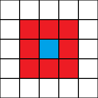
A popular example of cellular automaton is Conway’s game of life. In this case cells can assume the two states live or dead and are part of a two-dimensional grid. Every cell has therefore eight neighbours:

neighbours(c11) = { c00, c01, c02, c10, c12, c20, c21, c22 }

The transition function of Conway’s game of life can be summarised as follows:

  1. ∀c: Cell, such that c.statet = live ∧ 2 <= #alive_neighbourst(c) <= 3, we have c.statet+1 = live (“the cell survives”)
  2. ∀c: Cell, such that c.statet = dead∧ #alive_neighbourst(c) = 3, we have c.statet+1 = live (“the cell becomes alive”)
  3. For any other cell c for which neither 1 nor 2 above apply, we have c.statet+1 = dead (“if c is alive it dies, otherwise it stay dead”)

In the general definition of Cellular Automata nothing says that cells must be placed in a grid. In the remainder of this article we will write a Scala programme capable of computing the states of Cellular Automata based on binary trees. This programming challenge is described on website hackerrank.com: The Tree of Life Problem.

Cellular Automata on Binary Trees

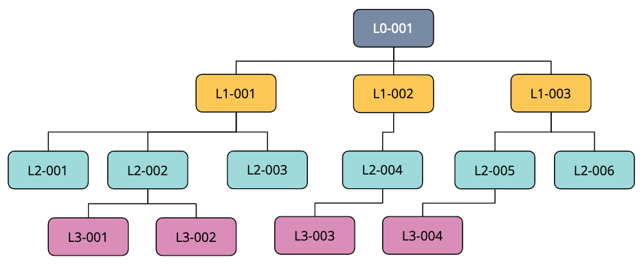
In this type of Cellular Automata cells live in a binary tree. The following picture exemplifies the concept:

Cell c0.0.0 is highlighted because I will use it to illustrate concepts such as the neighbours() function and the transition function.

Neighbours of a cell in a binary tree

The following picture shows what are the neighbours of cell c0.0.0 in the binary tree:

Definition – function neighbours() on a binary tree

The neighbours of a cell in a binary tree are:

  • its parent cell
  • its left child cell
  • its right child cell

If any of they neighbours listed above should not exist, a fictitious default cell is taken, whose state is false.

Definition – transition function f() on a binary tree

The transition function f: States4 -> State is a total function defined as follows:

∀c: Cell, c.statet+1 = f(c.statet, c.parent.statet, c.left-child.statet, c.right-child.statet)

Remark

c.parent, c.left-child, and c.right-child always return a cell, even if it is does not exist in the tree. Based on the definition above, in these cases a default cell with state false will be returned.

How can the transition function f be represented

A convenient way to model the transition function is through a table:

Transition function example

click on the image to enlarge it

Proposition – the number of possible transition functions for a cellular automaton in a binary tree is 2^16 = 65’536

This is obviously true in that there are 2^4=16 possible combinations of states for a cell and its neighbours, and for each such combination the transition function can assume one out of two values (live/dead).

Remark

In the table above, the mapping of columns to a cell and its neighbours determines an ordering. This choice corresponds with the specification of the sorting criterion defined for our programming exercise The Tree of Life Problem

Syntax for serialised cell binary trees

We now need to define the syntax in order to be able to read serialised binary tree from the command line. The grammar of a binary tree is simple and can be given like this using the Backus Naur form:

<node> ::= 'X' | '.'
<btree> ::= <node> | '('<btree>' '<node>' '<btree>')'

where:

  • ‘X’ signifies live, whereas ‘.’ signifies dead.
  • given a tree expression of the form “(expr1 expr2 expr3 )”, expr2 is the node, expr1 is its left child, and expr3 is its right child.

Examples

  1. X
  2. .
  3. (X . .)
  4. ((X . .) X (X . X))
  5. ((X . .) X (X . X)) X ((. X X) . (. X .))

Defining the transition function

Now that we know how to represent a CA binary tree, we need to define a suitable format for a transition function. All we need to consider is that a transition function is an ordered sequence of states of length 16. Given that states are live or dead, we can easily represent them as a 1 or a 0, respectively. Then, a convenient representation of a transition function is an integer n such that 0 <= n <= 65’535.

The Scala primitive type for an unsigned 16-bits integer is Char.

Reading the state of a particular node in a binary tree

Paths to a cell will be expressed relative to the root node. Every time the tree is traversed through the left sub-tree we will denote the move using character ‘<‘; when the right sub-tree is traversed we will use a ‘>’. Traversal paths will be delimited by square brackets. Examples:

  1. []
  2. [<]
  3. [><<><>>>]
  4. [<><]

where case 1 is the empty path and case 4 is illustrated by the following picture:

This syntax is arbitrary. One could as well write the paths above using characters ‘L’ and ‘R’ for left or right, respectively. We will use this syntax as specified by The Tree of Life Problem.

Historisation of past states

In order to solve the programming challenge we will need to historise the changes we apply to the tree every time we evolve it to the next generation by running the transition function as many times as requested. The number of times is expressed with a signed integer. The position in the history may be before the last element because, as we will see, time can go in the past.

Let us assume that:

  • The history has n generations (n trees whose states have been determined through subsequent applications of the transition function).
  • The current position in the history is m, with 0<= m <= n – 1 (history is 0-based)

If we are asked to apply the transition function t times, this is what our program must do:

  • if t >= 0 and m+t < n then m := t+m (move the current position ahead t times)
  • else if t >= 0 and m+t >= n then {
    • m := n-1 (move current position in history to the last one)
    • for i=1 to m + t – n + 1 {
      • apply transition function f to the tree at position m
      • add the tree resulting from point above to the history
      • move current position to the last one (tree just generated)
    • }
  • } else if t < 0 and m+t >= 0 {
    • m := m + t (go back in history t times)
  • } else ERROR

Examples

Historisation of past generartions

(click on the image above to enlarge it)

Input syntax

Input will be passed to the program through the command line.

  • The first line will be an integer expressing the transition function.
  • The second line will be a serialised cellular automaton binary tree.
  • The third line is an integer expressing the number of queries.
  • The subsequent lines will be as many as the number of queries as per the above.
  • Each query has the following syntax: <integer> <path expression>

The program must interpret the integer in the queries as explained above (Historisation of past states), read the state of the node denoted by the root-based traversal path in the same query, and print it to the standard output before processing the next query.

Example

23749
((X . .) X (X . X)) X ((. X X) . (. X .))
7
3 []
2 [><]
-1 [<>]
-1 [<><]
12 [<<<]
-2 [>><]
1 [>>>]

Assumptions

In this exercise we can safely assume that the traversal paths will be valid and that the history will not be explored before the start of time (generation zero).

We now have the conceptual framework required to start with the implementation. Let’s code!!!

Defining a node in the binary tree

sealed trait Status
object On extends Status
object Off extends Status
case class Node(s: Status) {
  override def toString = s match {
    case On => "X"
    case Off => "."
  }
}
object Node {
  val on = Node(On)
  val off = Node(Off)
}

At the moment of writing, website hackerrank.com supports Scala 2, not 3. This is why I have chosen a sealed trait with two objects instead of a simple enumeration to represent the state (Status in the code). In this way we have only two objects to represent the states. Object Status.On represents state live, whereas object Status.Off represents dead.

Class Node is trivial in that only has an attribute which is the state. Companion object Node returns two objects Node.on and Node.off with the obvious meaning. Please note that using objects like this guarantees that the number of instances in memory is strictly under control. If you do not know what is a companion object, please refer to http://www.scala-lang.org

Method toString() is overridden so that the string representation of the states matches the syntax requirements for this exercise.

Defining a cell

The definition of a node above may give the impression that there is no need to define yet another one for a cell. However, for reasons which will be clearer later, I will define a cell as a class with four attributes: a parent node, its own node, its left child node, and its right child node.

case class Cell(parent: Node, self: Node, left: Node, right: Node)

This definition will make the application of the transition function (the rule) simpler.

Defining a binary tree

Now that we have a node, we can easily define a binary tree.

case class BTree(n: Node, left:Option[BTree], right: Option[BTree])

A binary tree is defined as a structure formed by a node and two optional child trees. But before we delve deeper into the implementation of the BTree, we need to introduce the notion of a Rule.

Defining the rules

case class Rule(r: Char)

A rule is a Char. At this point you may be wondering why. The reason is that, as we have seen above, rules are sequences of 16 values (on/off, or live/dead, etc.). Char in Scala is an unsigned integer of exactly 16 bits. Therefore, it is an extremely compact way to encode a transition function (or a rule, using hackerrank’s terminology).

We can continue with the implementation of rules, by preparing useful data structures by means of the Rule companion object:

 object Rule {
      val nodeTypes = Vector(Node.off, Node.on)
      val sortedCells = nodeTypes.flatMap(n0 => nodeTypes.flatMap(n1 => nodeTypes.flatMap(n2 => nodeTypes.map(n3 => Cell(n0, n2, n1, n3)))))
      val ruleIndex: Map[Cell, Int] = sortedCells.indices.map(i => (sortedCells(i) -> i)).toMap
      val bits: Vector[Char] = (1 to 16).map(n => pow(2, n-1).toChar).toVector
    }

The above needs some explaining.

  • nodeTypes is an ordered sequence of node types modelled as a Vector (please note that no new instance of Node has been created, we are using the singletons defined above).
  • sortedCells is an ordered sequence of all the possible Cells created by generating all the combinations of off and on, and creating a Cell for each of them paying attention to the sort order defined by the author of this exercise who specifies that:
    • The state of the parent node comes first
    • The state of the left child node comes second
    • The state of the node whose new value we are computing comes third
    • The state of the right child node comes fourth
  • ruleIndex is a map which for every possible Cell returns the index of the value in the rule (please refer to the explanation above on how the rules are modelled).
  • bits is a Vector which for every bit index in the rule gives the corresponding binary representation of the on flag. For example, at position 0 it gives 0000000000000001. At position 1 it gives 000000000000010 and so on until position 15 where we have 1000000000000000.

We will better understand the use of the above when we will see how a rule is applied to a binary tree to evolve it to the next generation.

Applying a rule to a cell

case class Rule(r: Char) {
  def applyTo(c: Cell): Node = if ((bits(ruleIndex.getOrElse(c, -1)) & r) > 0) Node.on else Node.off
}

Let us assume that we are now applying a rule to a specific cell. Thanks to the plumbing above the implementation is trivial. First we look for the index in the rule where the new value of the cell is specified. In order to get this index we just have to use our map ruleIndex which contains all the possible cells (key) and their indexes (value). Once we know this index, we get the binary representation of an on flag (a 1) and we compute the logical AND of this flag with the value specified in the rule. If the result of this logical AND is different from 0 than the new state is on, otherwise it is off. This is illustrated by the following picture:

Rule applied to a cell

click on picture to enlarge

Remark

You will have noticed that I have used method getOrElse() and may be wondering why, given that by construction, I know that I will find my cell (given that ruleIndex contains all the possible cells). The reason is that the compiler does not know that the operation is safe because a get() on a map in general can fail. Therefore I return -1 in case the cell is not found (which cannot happen).

Applying a rule to the entire tree

case class BTree(n: Node, left:Option[BTree], right: Option[BTree]) {

     def applyRule(r: Rule, parent: Node = Node.off): BTree = {
       def nextCell(o: Option[BTree]) = o match {
         case Some(t) => t.n
         case None => Node.off
       }
       def subTree(o: Option[BTree]) = o match {
         case Some(t) => Some(t.applyRule(r, n))
         case None => None
       }
       BTree(r.applyTo(Cell(parent, n, nextCell(left), nextCell(right))), subTree(left), subTree(right))
     }

Method BTree.applyRule() above generates the next generation tree one node at a time by traversing itself recursively and computing the new state of each and every node.

Please note that the value of parameter parent is set to Node.off by default. This is useful because we start from the root of the tree which, by definition, does not have a parent node. You may wonder why than assign Node.off? The reason is that this is the desired behaviour specified by the author of this programming exercise. Let us now focus on the recursion. First, we need to identify the base case. Then, we must identify the recursion step. We will proceed using structural recursion. The base step is of course the node. We already know how to apply a rule to a node, we have seen it above. What we still need to add is that when a node does not have its parent (root) or one or two child nodes, we will assign default node Node.off. Again, this is the desired behaviour as per specs of this exercise. See The Tree of Life Pro for details (including discussion forums). The step is defined as follows: the new generation of:

BTree(n: Node, left: Option[BTree], right: Option[BTree])

is a new BTree having:

  • its node transformed by rule r: r.applyTo(Cell(parent, n, nextCell(left), nextCell(right)))
  • its sub trees t having node n recursively transformed applying rule r: t.applyRule(r, n)

Remarks

  • we use method def nextCell(o: Option[BTree]) to find the node of sub-trees, so that in case there is none, we can assign default value Node.off
  • we use method def subTree(o: Option[BTree]) to transform a sub-tree, because in case there is none, we just return None instead of starting a new recursive call

If you do not know what is Option[T] in Scala and the meaning of Some(), None, please refer to http://www.scala-lang.org

Now that we know how to transform a binary tree, we are ready to write a method which reads the state of any node given a correct root-based path expression.

Reading the state of a node

  case class BTree(n: Node, left:Option[BTree], right: Option[BTree]) {
     @tailrec
     final def readNode(path: List[Char]): Node = path match {
       case Nil => n
       case h :: pp => val next = h match {
           case '<' => left
           case '>' => right
           case _ => None
         }
         next match {
           case Some(t) => t.readNode(pp)
           case None => n
         }
     }
  }

Remark

We have seen above that the syntax of a path used in the queries is an arbitrary sequence of ‘<‘ and ‘>’ symbols enclosed by ‘[‘ and ‘]’. Method readNode() expects the path to be without any enclosing square brackets, only a sequence of ‘<‘ and ‘>’.

Method readNode() uses the character at the current position in the path to determine if the tree traversal must continue to the left or to the right, and proceeds recursively passing the path without the character just processed to the selected child tree.

Error management

  • if the path is empty than return the current node
  • if there is an unexpected character in the path (neither ‘<‘ nor ‘>’), than return the current node

Annotation @tailrec

You may have noticed that method readNode() has annotation @tailrec. If you do not know what it means, it is a property denoting recursive algorithms satisfying stricter conditions which allow the compiler to generate very efficient code, which makes the runtime performance of this type of recursion comparable to the performance of traditional loop control structures. In other words, you will not have to worry about the recursion running too deep and the method running out of stack. You may find better definitions of a tail recursive algorithm but, for the purposes of this article, I will just say that the intuitive notion entails ending the method with the recursive call. The recursive call is the very last thing which the method does.

Writing the parser

Above we said that the input has a syntax exemplified by this excerpt:

23749
((X . .) X (X . X)) X ((. X X) . (. X .))
7
3 []
2 [><]
-1 [<>]
-1 [<><]
12 [<<<]
-2 [>><]
1 [>>>]

Reading the rule is trivial:

val rule = Rule(readInt.toChar)

Reading the tree and the queries may be a little bit more involved.

Parsing the tree

@tailrec
def getTreeExpr(s: String, expr: String = "", depth: Int=0): (Option[String], String) = {
    if (s.isEmpty) (None, expr + s) else s(0) match {
      case '(' => getTreeExpr(s.substring(1), expr + s(0), depth + 1)
      case ')' => if (depth == 1) (Some((expr + s(0)).trim), s.substring(1))
                     else getTreeExpr(s.substring(1), expr + s(0), depth - 1)
      case c => if (Set(' ', 'X', '.').contains(c))
                  getTreeExpr(s.substring(1), expr + s(0), depth)
                else (None, expr + s)
    }
}

Method getTreeExpr() scans an input string one character at a time checking that only characters defined in the grammar of a tree expression are used (see section above) and that the brackets are balanced.

If a valid tree expression is recognised, it is returned as Some()[String], otherwise None is returned. The remaining part of the input string is also returned along with the recognised tree expression (or None in case of errors).

Please, note that the implementation of this method is also @tailrec.

Building the BTree from a valid tree expression

@tailrec
  def parseNode(s: String): (Option[Node], String) =
    if (s.isEmpty) (None, s) else s(0) match {
      case 'X' => (Some(Node.on), s.substring(1))
      case '.' => (Some(Node.off), s.substring(1))
      case ' ' => parseNode(s.substring(1))
      case _ => (None, s)
    }

  def parseTree(s: String): (Option[BTree], String) =
    if (s.isEmpty) (None, s) else parseNode(s) match {
      case (Some(n), rem) => (Some(BTree(n, None, None)), rem)
      case (None, _) => getTreeExpr(s) match {
        case (None, rem) => (None, rem)
        case (Some(exp), rem) => (BTree(exp), rem)
      }
    }

We will start with method readNode().

  • If symbol ‘X’ is encountered than Some(Node.on) is returned
  • If symbol ‘.’ is encountered than Some(Node.off) is returned
  • If symbol ‘ ‘ (a blank) is encountered than move on to the next char in the string
  • otherwise return None

Whatever the result of the scan, this method returns the remaining part of the input string.

Method parseTree()

  • if the input string is empty, return None
  • if the tree expression denotes a node n, return a BTree with node n and None as left and right sub-trees (leaf node)
  • if the tree expression is not a valid node, parse the input to check if it is a valid a tree expression
    • if not, return None and the input string
    • otherwise build a tree based on the valid tree expression using method def apply(s:String): Option[BTree]

Method def apply(s:String): Option[BTree]

object BTree {
     def apply(s:String): Option[BTree] =
      if (s.length < 7) parseNode(s) match {
          case (Some(n), _) => Some(BTree(n, None, None))
          case _ => None
      } else (s(0), s(s.length - 1)) match {
        case ('(', ')') =>
          val (left, lRem) = parseTree(s.substring(1, s.length - 1))
          val (node, nRem) = parseNode(lRem)
          val (right, rRem) = parseTree(nRem)
          (node, left, right) match {
            case (Some(n), Some(l), Some(r)) => Some(BTree(n, Some(l), Some(r)))
            case _ => None
          }
        case _ => None
      }
  }

Before explaining method apply() it is worth noting that it uses method parseTree() which, as we have seen above, uses method apply(). This situation is called mutual recursion which for a functional programmer is the place “where eagles dare”.

Method apply() uses convenience methods parseNode() and parseTree() to deconstruct a serialised binary tree. From the grammar introduced above we know that a tree is represented as a triplet where the first part is the optional left child tree, the second one is the current node, and the last one is the optional right tree. In order to determine whether the input string must be parsed as a plain node or a binary tree, this method uses a cheap trick: checks the length. This works because we know that the simplest tree is formed by all nodes and has a form similar to “(X . X)” which are seven characters: left bracket, node symbol, blank, node symbol, right bracket. There may be more elegant ways to implement this part, but this works pretty well and is efficient so, for the purposes of this exercise, I will not try to do any better. But, of course, you can!

The apply() method proceeds with structural recursion: if a proper tree expression is recognised, its left and right sub-trees are recursively inspected, until the entire expression is processed, or an error is encountered.

We are now ready for the implementation of the parser for the queries.

Parsing the queries

We have seen above that queries have syntax exemplified by these expressions:

3 []
2 [><]
-1 [<>]
-1 [<><]
12 [<<<]
-2 [>><]
1 [>>>]

Parsing the first part is trivial: it is a signed integer. More interesting is parsing the second part. Here, I will use a regular expression.

def parseQuery(s: String): (Int, String) = {
    import scala.util.{Failure, Success, Try}
    val params = s.split(" ")
    if (params.length != 2) (0, "")
    else {
      val n = Try(params(0).toInt) match {
        case Success(n) => n
        case Failure(_)  => 0
      }
      val regex = "^\\[[<>]*\\]$".r
      val path = if (regex.matches(params(1))) params(1).substring(1, params(1).length-1)
                 else ""
      (n, path)
    }
  }
  • the query is first split using blank as the separator
  • the conversion of the first token to Int is then attempted using functional construct Try instead of imperative exception handling.
  • if the path expression is correct, the enclosing square brackets are removed. This is achieved using params(1).substring(1, params(1).length-1) which omits the first and last character.

Processing the input

def main(args: Array[String]): Unit = {
    val rule = Rule(readInt.toChar)
    BTree(readLine()) match {
      case Some(t) =>
        val nrQueries = readInt()
        assert(nrQueries > 0)
        processInput(nrQueries, rule, Hist(t))
      case None => System.exit(-1)
    }
  }

Method main() is very simple. First, it reads the rule and saves it as a Char. Then, it reads the serialised tree and tries to build a BTree based on it. The test cases run by hackerrank are guaranteed to be syntactically correct. So, we do not have to worry about invalid tree expressions.

After that, the number of queries is read. The core of the algorithm is implemented in method  def processInput(nQueries: Int, rule: Rule, acc: Hist): Unit

@tailrec
  def processInput(nQueries: Int, rule: Rule, acc: Hist): Unit = if (nQueries > 0) {
      val (offset, path) = parseQuery(readLine())
      val h = perform(offset, rule, acc)
      println(h.hist(h.ix).readNode(path.toList).toString())
      processInput(nQueries - 1, rule, h)
  }

This method runs nQueries times and every time reads a query from the command line, processes it, and prints the result to the standard output.

Remark

In imperative languages, instead of writing tail-recursive method processInput() one would have written a simple loop (for or while) using modifiable data structures. The beauty of functional programming is that we can write equivalent code to the imperative which is equally efficient (being @tailrec) without dangerous side effects thanks to the use of immutable data.

Before looking into the perform() method we need to see how the history is implemented and how it works.

The history class

case class Hist(ix: Int, hist: Vector[BTree])
  object Hist {
    def apply(t: BTree): Hist = Hist(0, Vector(t))
  }

We have seen above how the generations of transformed trees are persisted. This data structure contains all the transformations up to the previous generation, along with the position in the history. This is necessary because queries may require us to go back to the past (but not beyond generation 0)

Please note the convenience method apply() which, given a BTree, builds a history object initialised with this tree and an index at position 0.

Method perform()

 def perform(offset: Int, rule: Rule, h: Hist): Hist = {
    assert(h.hist.nonEmpty)
    @tailrec
    def run(times: Int, acc: Vector[BTree] = Vector.empty[BTree]): Vector[BTree] =
      if (times < 1) acc
      else run(times - 1, acc :+ acc.last.applyRule(rule))

    val newIx = h.ix + offset

    if (newIx < 0) h
    else if (newIx < h.hist.length) Hist(newIx, h.hist)
    else Hist(newIx, run(offset - (h.hist.length - h.ix - 1), h.hist))
  }
  • If the offset requires us to move to a position beyond the end of the existing history, method perform will apply the rule to the latest tree as many times as is required to fill the gap in the history.
  • If instead the offset falls within the history, the entire history is returned, along with the new position determined by adding the offset to the previous position.

The updated history returned by method perform() allows method processInput() to print the result to the standard output using this simple statement: println(h.hist(h.ix).readNode(path.toList).toString())

This completes the explanation of the implementation. I hope you have enjoyed this article and have learned something useful. If you have found mistakes you can let me know using the contact form. Please consider that this article and the source code are provided as is. I write this content to the best of my knowledge but there is no guarantee that it is correct or otherwise suitable for any purpose.

Code of conduct

This content aims at making you a better programmer, but you may not use it to gain undeserved credits in programming challenges on any web site. If you want to take programming challenges, please write your own code and do not copy and paste this code because it is against the code of conduct.

Ok, enough with burocracy

If you came this far with this article you deserve a little treat. Here is my code on github:

https://github.com/maumorelli/alaraph

Thank you for reading and up Scala!!!

Matrix Rotation – Functional Implementation in Scala

Introduction

Matrix rotation is the transformation based on replacing the value of a cell with the value of an adjacent one, where the notion of “adjacent” is expressed with reference to the decomposition of a matrix in “rings”. It’s a bit like peeling an onion. Let us consider the matrix depicted above. We can easily identify its outer ring. { a00, a01, a02, a03, a04, a14, a24, a34, a33, a32, a31, a30, a20, a10 }. The next ring is also easily identified: { a11, a12, a13, a23, a22, a21 }.

Assumptions

In this article I will assume that matrix rotation is applied counterclockwise. Similar arguments apply if the rotation is done clockwise. For simplicity’s sake, I will use a matrix of integers.

Representing a matrix

The typical representation of a matrix is based on two-dimensional arrays. Since we will use Scala and we want to learn to write clean algorithms without side effects, we will use immutable type Vector instead.

So, our matrix of integers will be defined as matrix: Vector[Vector[Int]]

The algorithm

I will illustrate the algorithm in steps. First will I explain how the decomposition of a matrix in rings simplifies the logic of rotation. Second, I will explain how to implement this logic without duplicating the content of the matrix for the creation of its constituent rings: we will create an abstraction which will allow us to navigate the matrix as if it were structured in rings. This trick will reduce the space complexity of the algorithm.

Using the rings to implement rotation

Given the matrix in our example above, we can represent the rings using vectors:

val ring0 = Vector( a00, a01, a02, a03, a04, a14, a24, a34, a33, a32, a31, a30, a20, a10 )

val ring1 = Vector( a11, a12, a13, a23, a22, a21 )

As you can see, we have ring0.size = 14 and ring1.size = 6

The logic of rotation can now be expressed using plain modulo arithmetic. If we define “r” the number of (anticlockwise) rotations, and “i” the position of a cell in vector ring0, the new value of ring0(i) is the value of cell ring0((i+r) % ring0.size)

Let us now set r=1

ring0(0) = ring0((0+1) % 14) = ring0(1) = a01

ring0(1) = ring0((1+1) % 14) = ring0(1) = a02

ring0(13) = ring0((13+1) % 14) = ring0(0) = a00

The logic above can be written like this:

(0 until ring0.size).map(i -> ring0((i+r) % ring0.size))

where the “map” method applies the function passed to it as an argument to each element of the collection.

If we apply the logic above to each ring of the matrix, we obtain the rotated matrix.

Implementation

Given a matrix, we have seen above that we can conceptualise it as a set of concentric rings (remember the onion metaphor). We will now write our first method, which will generate a Vector allowing to navigate the matrix as a ring of depth “r”, where depth is 0 for the outer ring.

def m2ring(matrix: Vector[Vector[Int]])(offset:Int): Vector[(Int, Int)] = {
    val m = matrix.size
    val n = matrix(0).size
    val north = (0 + offset to n - 1 - offset).map(j => (offset, j)).toVector
    val east = (1 + offset to m - 2 - offset).map(j => (j, n - 1 - offset)).toVector
    val south = (n - 1 - offset to 0 + offset by -1).map(j => (m - 1 - offset, j)).toVector
    val west = (m - 2 - offset to 1 + offset by -1).map(j => (j, offset)).toVector
    north ++ east ++ south ++ west
  }

If we invoke method m2ring passing our example matrix above, with offset = 0 (this is how the ring depth is called in the method signature), we get this output:

Vector( (0,0), (0,1), (0,2), (0,3), (0,4), (1,4), (2,4), (3,4), (3,3), (3,2), (3,1), (3,0), (2,0), (1,0) )

If we invoke m2ring(matrix)(1) we get:

Vector( (1,1), (1,2), (1,3), (2,3), (2,2), (2,1) )

Our next method will invoke m2ring for each ring depth until the entire matrix is processed (the entire onion is peeled). This method will return two data structures:

  • A Vector of vectors. This vectors will have as many elements as there are rings in the matrix. For each ring, say “i”, rings(i) is the vector having as many elements as there are cells in ring “i”, each element being the (row, col) coordinates of the cell in the matrix.
  • A map having key (row, col) and value (index1, index2) where:
    • (row, col) are the coordinate of a cell in the matrix
    • index1 is the index of the rings vector corresponding to the ring where cell (row, cell) belongs
    • index2 is the index of vector rings(index1) corresponding to the position of cell (row, cell)
def m2rings(matrix: Vector[Vector[Int]]) = {
    val m = matrix.size
    val n = matrix(0).size
    val g = m2ring(matrix)(_)
    val rings = (0 to Math.min(m,n)/2-1).map(i => g(i))
    val coords = (0 until rings.size).flatMap ( i => (0 until rings(i).size).map ( j => rings(i)(j) -> (i, j))).toMap
    (rings, coords)
  }

If we invoke m2rings passing our example matrix above we obtain:

rings = Vector(Vector( (0,0), (0,1), (0,2), (0,3), (0,4), (1,4), (2,4), (3,4), (3,3), (3,2), (3,1), (3,0), (2,0), (1,0) ), Vector( (1,1), (1,2), (1,3), (2,3), (2,2), (2,1) ) )

coords = Map ( (0,0) -> (0,0), (0,1) -> (0,1), (0,2) -> (0,2), (0,3) -> (0,3), (0,4) -> (0,4), (1,0) -> (0,13), (1,1) -> (1,0), (1,2) -> (1,1), (1,3) -> (1,2), (1,4) -> (0,5), (2,0) -> (0,12), (2,1) -> (1,5), (2,2) -> (1,4), (2,3) -> (1,3), (2,4) -> (0,6), (3,0) -> (0,11), (3,1) -> (0,10), (3,2) -> (0,9), (3,3) -> (0,8), (3,4) -> (0,7) )

We have now all the elements to implement the matrix rotation method:

  def perform(matrix: Vector[Vector[Int]], times: Int) = {
    val (rings, coords) = m2rings(matrix)
    def rotateMatrix(lmat: List[Vector[Int]], acc: Vector[Vector[Int]], row: Int = 0): Vector[Vector[Int]] = lmat match {
      case Nil => acc
      case r::rr =>
        val rotatedRow = (0 until r.size ).map { case col =>
                      val (rix, vix) = coords.getOrElse((row, col), (0,0))
                      val (_r, _c) = rings(rix)((vix+times) % rings(rix).size)
                      matrix(_r)(_c)
                    }.toVector

        rotateMatrix(rr, acc :+ rotatedRow, row + 1)
    }
    rotateMatrix(matrix.toList, Vector.empty, 0)
  }

The complete source code for this algorithm is available on my github space.

I hope you enjoyed this article and, up Scala!!!

Solving the Klotski puzzle in Scala

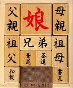
https://upload.wikimedia.org/wikipedia/commons/8/84/Hakoiri3.jpg

Klotski puzzle, Wikimedia

A very good description of the Klotski puzzle is available on programming website Hackerrank. A brief description is given here for convenience’s sake.

What is Klotski

Klotski is a puzzle consisting in a rectangular board containing labelled blocks. These blocks can slide in the four directions up/down/left/right, but they can neither overlap, nor exit the board.

One of these blocks is called the target. Objective is to find the shortest sequence of moves (path) allowing to place the target block in a given location. Any equally short sequence is deemed equivalent.

In counting the moves, subsequent slides of the same block are all counted as one move.

Why is Klotski a challenging programming problem?

Solving the problem requires the ability to reduce unnecessary intermediate configurations which would otherwise lead to a fast explosion of cases to be examined. Although the problem remains intrinsically hard, it is possible to implement optimised algorithms able to solve puzzles requiring n < 200 moves. I tried to find mathematically rigorous proofs of the complexity of known Klotski solver algorithms, but I could not find one. Or at least, none was proved.

The required optimisations to tackle puzzles of the complexity explained above are a very good learning opportunity for programmers who want to learn algorithms, functional programming, recursion, hashing, and many more skills. I have chosen Scala to solve the problem because it allows to write code without side effects, which is particularly suited to teaching good programming practices.

Let’s start from the data structures

I will introduce some basic terms. The picture below represents a Klotski board with five blocks (A, B, C, D, and E). Empty cells are denoted with “.” characters.

Labels need not be single letters, they can be arbitrary strings. If labels have length L > 1, empty cells are denoted by sequences of L “.” characters. For example, the board depicted below is equivalent (isomorphic) to the board above.

We will start from the representation of a Cell.

 case class Cell(y: Int, x: Int) {
    def applyOffset(o: Offset) = Cell(y + o.dy, x + o.dx)
    override def toString = "(%d,%d)".format(y, x)
  }

Cell is a case class and this allows us to write expressions like Cell(2, 3) without having to explicitly invoke a constructor. I have overridden the “toString” method bacause I want an object like Cell(2, 3) to be rendered as “(2, 3)” instead of the default “Cell(2, 3)”. Additionally, I have defined method “applyOffset” which not surprisingly applies an offset to a Cell.

Remark

Please note that Scala is (also) a functional language and the philosophy is to have immutable objects. Therefore, applying an offset to a Cell creates a new Cell, leaving the original one unchanged.

Similarly, we define case class Offset.

  case class Offset(dy: Int, dx: Int) {
    def invert = Offset(-dy, -dx)
  }

This is a trivial class which I will not comment further. A slightly more interesting class is Board.

  case class Block(symbol: String, cells: Set[Cell]) {
    private def minmaxXY = {
      val xx = cells.map { case Cell(_, x) => x }
      val yy = cells.map { case Cell(y, _) => y }
      (xx.min, xx.max, yy.min, yy.max)
    }

    val (minX, maxX, minY, maxY) = minmaxXY
    val uL = Cell(minY, minX)
    val bR = Cell(maxY, maxX)
    val width = maxX - minX + 1
    val height = maxY - minY + 1
  }

A Block is modelled as a set of cells, labelled with a symbol.

Method “minmaxXY” extracts the maximum and minimum X and Y coordinates from the cells. Val xx is built by extracting only the x coordinate from each Cell. The same applies to val yy, mutatis mutandis. An important derived attribute, which we will use to denote the position of a block, is its upper left corner, “uL”.

Remark

It is important to notice that the “uL” cell need not be inside the block itself. For example, let us consider L-shaped block A below. Its upper left cell is Cell(0, 0) which does not belong to the block Block(“A”, Set(Cell(0, 1), Cell(1, 1), Cell(2, 0), Cell(2, 1))

  0 1 2 3 
0 . A . .
1 . A . .
2 A A . .
3 . . . .

We will now model the concept of a move: when a block slides from a certain position to another position, we will log these bits of information:

  • Symbol
  • Upper left cell of the starting position
  • Upper left cell of the ending position

Let us make an example. In the board below we will slide block A:

  0 1 2 3        0 1 2 3
0 . A . .      0 . . . A
1 . A . .  =>  1 . . . A
2 A A . .      2 . . A A
3 . . . .      3 . . . .

The move will be represented with Move(“A”, Cell(0, 0), Cell(0, 2).

case class Move(block: String, from: Cell, to: Cell) {
    def offset = Offset(to.y - from.y, to.x - from.x)
  }

Case class Move has method “offset” which allows to derive the offset applied to Cell “from” to get to Cell “to”.

Building a Board

A board is given in input as a text. The format is illustrated with an example:

5 4
. A B B
. A B B
A A C .
D D C .
D . . E

On the first row we have the number of rows and the number of columns (5 and 4 respectively). Every cell is represented by its symbol and cells are spaced with a blank. We are now ready to define case class Board.

case class Board(blocks: Map[String, Block], block:String, maxX: Int, maxY: Int) {
    val minX = 0
    val minY = 0
    val symbols = blocks.keys
    ...
}

A Board is a map of symbols pointing to their respective block. The special block is saved in property “block”. maxY and maxX have the obvious meaning, but remember that the count starts from 0. In order to create a Board starting from the text input we will create a builder method in the companion object. Remember that in Scala every class can have a companion object with the same name, which is a singleton. See Scala’s documentation on http://www.scala-lang.org for more details.

  object Board {
    def build(b: Vector[Vector[String]], block:String) = {
      val maxY = b.size - 1
      val maxX = b(0).size - 1
      val eb = "." * b(0)(0).length //empty block
      val flatb = for { i <- 0 to maxY
                        j <- 0 to maxX
                        if b(i)(j) != eb
      } yield (b(i)(j), Cell(i,j))

      Board(flatb.groupBy(_._1).map {
        case (y, zz) => (y, Block(y, zz.map(_._2).toSet))
      }, block, maxX, maxY)
    }
  }

“maxY” is set to the number of rows minus 1 (0-referenced). Likewise, “maxX” is set to the number of columns minus 1. Constant “eb” is built by concatenating as many times the “.” character as the length of the symbols in this particular board. The “for” loop goes through the Vector and for every Cell with a symbol different than the empty cell, yields a tuple containing the symbol and the Cell where the symbol was found. The result of this scan is saved in value “flatb”. If we take our example above (copied here for convenience’s sake), this will be the result:

. A B B
. A B B
A A C .
D D C .
D . . E
val flatb = Seq[("A", Cell(0, 1)), ("B", Cell(0, 2)), Cell("B", Cell(0, 3)),
                ("A", Cell(1, 1)), ("B", Cell(1, 2)), Cell("B", Cell(1, 3)),
                ("A", Cell(2, 0)), ("A", Cell(2, 1)), Cell("C", Cell(2, 2)),
                ("D", Cell(3, 0)), ("D", Cell(3, 1)), Cell("C", Cell(3, 2)),
                ("D", Cell(4, 0)), ("E", Cell(4, 3))]

What do we need to do to get from the above to the format required to build a block? Function “groupBy” is the answer. See how it works.

flatb.groupBy(_._1).map {
case (y, zz) => (y, Block(y, zz.map(_._2).toSet))
}

Let’s do it step by step.

flatb.groupBy(_._1)= Map[("A", IndexedSeq[("A", Cell(0, 1)), 
                                          ("A", Cell(1, 1)), 
                                          ("A", Cell(2, 0)), 
                                          ("A", Cell(2, 1))]),
                         ("B", IndexedSeq[("B", Cell(0, 2)), 
                                          ("B", Cell(0, 3)), 
                                          ("B", Cell(1, 2)), 
                                          ("B", Cell(1, 3))]),
                         ("C", IndexedSeq[("C", Cell(2, 2)), 
                                          ("C", Cell(3, 2))]),
                         ("D", IndexedSeq[("D", Cell(3, 0)), 
                                          ("D", Cell(3, 1)), 
                                          ("D", Cell(4, 0))]),
                         ("E", IndexedSeq[("E", Cell(4, 3))])                                  

The subsequent invocations of the “map” method do the following:

  • Create a Block based on each symbol and the sequence of Cells of which the block is composed
  • Convert sequences of Cells into sets of Cells

Performing a move

Performing a move means to slide a block in one of the four admissible directions up/down/left/right. However, some moves are invalid:

  • Moves taking a block out of the board
  • Moves making a block overlap with other blocks

We will now implement the “perform” method which will demonstrate how efficient is the chosen data structure for the definition of the required logic.

 case class Board(blocks: Map[String, Block], block:String, maxX: Int, maxY: Int) {
    val minX = 0
    val minY = 0
    val symbols = blocks.keys

    def perform(s: String, o: Offset) = {
      val b = blocks(s)
      val cells = b.cells.map(c => c.applyOffset(o))
      val outOfBound = cells.find { case Cell(y, x) => y < 0 || y > maxY || x < 0 || x > maxX }

      outOfBound match {
        case Some(_) => None
        case None => val otherBlocks = blocks - s
          val overlap = otherBlocks.values.find(_.cells.intersect(cells) != Set.empty)
          overlap match {
            case Some(_) => None
            case None => Some(Board(blocks + (s -> Block(s, cells)), block, maxX, maxY))
          }
      }
    }
  (...)
 }

Given a Board b, performing a move requires the specification of which block we want to move and in which direction. The block is denoted by its symbol. The direction of the move is denoted by the equivalent offset. The four cardinal directions are denoted by the following offsets:

One move to the left  => Offset( 0, -1)
One move to the right => Offset( 0,  1)
One move upwards      => Offset(-1,  0)
One move downwards    => Offset( 1,  0)

Lets us now consider our example again. Let “brd” be the board depicted below.

. A B B
. A B B
A A C .
D D C .
D . . E

brd.perform(“C”, Offset(0, 1))

will generate this new board:

. A B B
. A B B
A A . C
D D . C
D . . E

Line 8 of code snipped above applies the offset to every cell belonging to the moving block. Line 9 checks whether or not cells exist which after the move go out of the board. In the affirmative case, the result of the move is Option.None (if you do not know what is Option in Scala, please refer to http://www.scala-lang.org).

The second and last check is whether or not the cells of the moved block overlap with the cells of any other block. Please note that the overlap check is elegantly implemented with the Set.intersect method. If the move succeeds, the perform method returns Some(Block).

For the moment we will leave the implementation of class Board. Later in this paper I will come back to it because we will see a magic one-liner which will make the difference between failing and succeeding the demanding performance requirements tested by http://www.hackerrank.com. This single one liner has costed me sleepless nights 🙂

Resist the temptation to look ahead, we have a lot more funny stuff before then.

Laying the ground for the algorithmic approach

I will use this paper to teach you how to write recursive code in Scala, which is an integral part of the functional programming approach. Please note that although recursion has a bad reputation in imperative languages because it consumes precious resources like the stack, the Scala compiler can generate very efficient code, virtually as efficient as a while cycle, on condition that recursion is “tail recursion”, that is, the statement invoking the same method is the very last statement of the method. If you learn to think in terms of recursion, you will be able to write clean code without side effects which uses primarily unmodifiable data. One of the key data structures every Scala programmer must master is List. We will now show how to use lists as a foundational block in our functional approach to solving Klotski. But before then, we need to model the internal states of the Klotski solver. We will now consider the following example.

3 3
A . B
C . B
C D .
A
2 2

The example above has the same syntax we have already described, except for the last two rows, which specify the target: move block “A” to position Cell(2, 2) with the lowest number of moves.

For each configuration our algorithm will do the following:

  • For every symbol, move it around in every possible direction until no more valid moves are possible, avoiding duplicate states (if a move gets to a board which was already generated, the move is discarded)
  • When moving the special block, check if the board is a solution to the problem
  • Add every new board to the history
  • Add all new board generated during this step to the set of boards which have to be explored at the next iteration.

Proposition

The first board generated which is a solution to the puzzle, is the shortest path to the solution.

Since we are exploring the space of solutions stepwise (every step increases the number of moves of one unit), the proposition is trivially true.

Remark

Above we observed that at every step we must add the new boards generated to the set of boards which have to be explored at the next iteration. However, this is not enough. We have a gap in our data model in that, in order to describe the solution, we also need to save the path to each board (the sequence of moves which brings us from the initial board to the desired state in the minimum number of steps. We will call this object a Trail and we will define it as a Board and the Path which has generated it starting from the initial position. Before giving the details, I will show an excerpt of the internal states of our solver. Numbered boards are our “history”. At each iteration, for every symbol all possible moves are tried, avoiding duplicates. This will proceed recursively, as we will see.

1 Move
                                          
A . B       Move(A,(0,0),(0,1))    . A B
C . B  (0) --------------------->  C . B  (1)
C D .                              C D .

A . B       Move(A,(0,0),(1,1))    . . B
C . B  (0) --------------------->  C A B  (2)
C D .                              C D .

A . B       Move(B,(0,2),(0,1))    A B .
C . B  (0) --------------------->  C B .  (3)
C D .                              C D .

A . B       Move(B,(0,2),(1,2))    A . .
C . B  (0) --------------------->  C . B  (4)
C D .                              C D B

A . B       Move(D,(2,1),(1,1))    A . B
C . B  (0) --------------------->  C D B  (5)
C D .                              C . .

A . B       Move(D,(2,1),(0,1))    A D B
C . B  (0) --------------------->  C . B  (6)
C D .                              C . .

A . B       Move(D,(2,1),(2,2))    A . B
C . B  (0) --------------------->  C . B  (7)
C D .                              C . D

2 Moves

. A B       Move(B,(0,2),(1,2))    . A .
C . B  (1) --------------------->  C . B  (8)
C D .                              C D B

. A B       Move(C,(1,0),(0,0))    C A B
C . B  (1) --------------------->  C . B  (9)
C D .                              . D .

. A B       Move(D,(2,1),(1,1))    . A B
C . B  (1) --------------------->  C D B  (10)
C D .                              C . .

. A B       Move(B,(2,1),(2,2))    . A B
C . B  (1) --------------------->  C . B  (11)
C D .                              C . D

(..............................................)

Solution:

A . B   Move(A,(0,0),(1,1))   . . B
C . B --------------------->  C A B
C D .                         C D .

. . B   Move(C,(1,0),(0,0))   C . B
C A B --------------------->  C A B
C D .                         . D .

C . B   Move(D,(2,1),(2,0))   C . B
C A B --------------------->  C A B
. D .                         D . .

C . B   Move(A,(1,1),(2,2))   C . B
C A B --------------------->  C . B
D . .                         D . A

Let us now define the Trail and other useful types.

    case class Trail(board: Board, path: Path)
    type Trails = List[Trail]
    type Offsets = List[Offset]

The Klotski solver algorithm

Based on what we have seen above, the solver is a breadth-first visit of the solution space which explores each individual board generating all the admissible moves symbol by symbol, discarding duplicate states. We can visualize it as a tree whose nodes are Trails (a Board with its Path).

This is the tree of internal states of the solver. Every level down is one more move in the path.

A very handy representation of a breadth-first approach is a list where every subsequent Trail has path with length equal or greater than the one before. In our recursive algorithm it will be built by appending new Trails to the existing list of Boards to be explored.

This is a list representation of the breadth-first visit of the tree. Lists come handy in Functional Programming because they are recursive data structures.

Time has come to read some code.

  def solve(brd:Board, block:String, target:Cell):Path = {
    val symbols = (brd.symbols.toSet - block).toList
    val hist = scala.collection.mutable.Set[Int]()
    val offsets = List(Offset(-1, 0), Offset(1, 0), Offset(0, -1), Offset(0, 1))
    case class Trail(board: Board, path: Path)
    type Trails = List[Trail]
    type Offsets = List[Offset]
 
    (...)

    def _solve(trails: Trails): Path = trails match {
      case t :: tx => val (_trails, _path) =  if (t.path == Nil || 
        t.path.head.block != block) pursueTarget(List(t))
      else (Nil, Nil)
        if (_path != Nil) _path
        else {
          val _symbols =  if (t.path == Nil) symbols
          else (symbols.toSet - t.path.head.block).toList
          val newTrails = checkOneTrail(t, _symbols)
          _solve(tx ++ newTrails ++ _trails)
        }
      case Nil => Nil
    }


    if (isSolved(block, target, brd)) Nil
    else {
      hist.add(brd.hashCode)
      val trails = List(Trail(brd, Nil))
      if (!symbols.isEmpty) _solve(trails) else pursueTarget(trails)._2
    }
  }

The algorithm is driven by the “solve” method, which is invoked passing the Board, the special block symbol, and the target Cell. The “solve” method checks if by chance the initial Board is already a solution (border case). Otherwise it adds the “hashCode” of the Board to the “hist” Set.

The history of explored Boards

I initially implemented the “hist” Set using a more “functional” immutable Set passed as a parameter to “_solve” and all other methods. In this case, however, given the fast increasing size I then consciously decided to compromise on the purity of the implementation to optimise the performance. Since the “hist” Set is only visible inside method “solve”, the risk of undesired side-effects is well controlled. This is an example of how first principles can be consciously traded off if one knows what he/her is doing.

But this is not all. A second design decision is to historise hash codes of the Boards, instead of the Boards themselves. The rationale is again performance (www.hackerrank.com requirements in this regard are strict). It is a lot more efficient to compare integers than to compare entire boards and their blocks, symbols and cells. Of course, the probability of a clash is small when using good hashing algorithms, but its not null (for the very nature of hashes, which generate values in a constrained range from unconstrained inputs). This is the trade-off. It works in practice, but it is not a 100% mathematically sound approach. So, what would happen in case of a clash? A board would be “found” in the history, which was never before really generated and in the worst scenario this could lead to a sub-optimal solution. This never occurred in any of the 26+ http://www.hackerrank.com test cases or even in my own ones.

The hash function

This function is a very critical part of the algorithm: getting it wrong screws up everything else (I am saying it for a reason). So, what’s special about the hash function of a Board and why does not the default “hashCode” function work well enough? The default hashCode implementation in Scala is actually pretty good. But when we run the algorithm using the default implementation we have an exponential explosion of states. I will now illustrate why and how to fix it. Let us consider the following Klotski puzzle.

5 4
A B C .
A D E .
F F G G
F . G .
H I L L
A
3 3

The following Boards all have distinct hashCodes, because they are different. But, are they any different in terms of solving the puzzle? No, they are not, because they have the same exact morphology the only distinction being that same-shaped blocks have different labels, which is not a differentiator for the search of the optimal path.

A B C .   A C B .   A B C .   A B C .   A B C .
A D E .   A D E .   A E D .   A D E .   A D E .
F F G G   F F G G   F F G G   G G F F   F F G G
F . G .   F . G .   F . G .   G . F .   F . G .
H I L L   H I L L   H I L L   H I L L   I H L L

I could list many more equivalent permutations of this Board, but by now you should get the point. So, our hash function will need to generate the same code for all the equivalent Boards, so that they are not unnecessarily explored slowing down the search to unacceptable levels. Or, if you prefer, so that the space of possible solutions is limited to truly relevant configurations. This is how the correct “hashCode” method looks like.

override def hashCode = (blocks(block).hashCode :: (blocks - block).values.map (b => b.cells.hashCode).toList.sorted).hashCode

The equivalent blocks are made to generate the same hash by removing their symbol from the computation. The symbol of the special block is instead maintained because where the special block is located is a differentiating factor. This hashCode function induces an equivalence relation on the set of generated Boards. Reducing the search to the set of equivalence classes makes the complexity of the search manageable with problems of the size defined above (but remains inefficient for problems of arbitrary size).

Coming back to the algorithm, at the core of the “solve” method there is this logic:

  • A trail is explored to see if it is possible to move the special block to the target cell. In the affirmative case the algorithm stops and returns the path.
  • Otherwise, the new configurations are added to the history and are appended to the set of Boards which have to be further explored.
  • The trail is processed by scanning all possible moves of all symbols in order to prepare the boards to be explored at the next iteration. These new configurations are appended to the list of trails to be explored. This sequence is guaranteed to produce a list equivalent to a breadth-first tree traversal (see above).
  • Some further optimisations are applied. For example, if the last move in the path of a given trail involved symbol s, the algorithm will not try to move block s because all possible moves were already tried in the step before.

The below is the implementation of all the other recursive parts of the algorithm, which should be self-explanatory after all the clarifications above.

  def solve(brd:Board, block:String, target:Cell, maxmoves: Int = 250):Path = {
    val symbols = (brd.symbols.toSet - block).toList

    val offsets = List(Offset(-1, 0), Offset(1, 0), Offset(0, -1), Offset(0, 1))
    case class Trail(board: Board, path: Path)
    type Trails = List[Trail]
    type Offsets = List[Offset]


    def moveBlockAroundOnce(trail: Trail, s: String, offsets: Offsets, hist: Set[Board]=Set.empty, acc: Trails = Nil): Trails = offsets match {
      case o :: ox => trail.board.perform(s, o) match {
        case Some(newBoard) => if (hist.contains(newBoard))
          moveBlockAroundOnce(trail, s, ox, hist, acc)
        else
          moveBlockAroundOnce(trail, s, ox, hist+newBoard, Trail(newBoard,
            Move(s, trail.board.blocks(s).uL, newBoard.blocks(s).uL) :: trail.path)::acc)

        case None => moveBlockAroundOnce(trail, s, ox, hist, acc)
      }
      case Nil => acc
    }

    def moveBlockAround(trails: Trails, s: String, hist: Set[Board]=Set.empty, acc: Trails = Nil): Trails = trails match {
      case t :: tx => val _trails = moveBlockAroundOnce(t, s, offsets, hist + t.board)
        moveBlockAround(tx ++ _trails, s, hist.union(_trails.map(t=>t.board).toSet), acc ++ _trails)
      case Nil => acc
    }

    def sanitize(trails:Trails, acc: Trails = Nil): Trails = trails match {
      case t::tx => val hashcd = t.board.hashCode
        if (hist.contains(hashcd)) sanitize(tx, acc)
        else {
          hist.add(hashcd)
          sanitize(tx, t::acc)
        }
      case Nil => acc
    }

    def checkOneTrail(trail: Trail, symbols: List[String], acc: Trails = Nil): Trails = symbols match {
      case s :: sx => val _trails = moveBlockAround(List(trail), s)
        val newTrails = sanitize(_trails)
        checkOneTrail(trail, sx, acc ++ newTrails)
      case Nil => acc
    }

    def pursueTarget(trails: Trails, acc: List[Trail] = Nil): (Trails, Path) = trails match {
      case t :: tx => if (isSolved(block, target, t.board)) (trails, t.path)
      else {
        val _trails = moveBlockAroundOnce(t, block, offsets)
        val newTrails = sanitize(_trails)
        pursueTarget(tx ++ newTrails, acc ++ newTrails)
      }
      case Nil => (acc, Nil)
    }

    def _solve(trails: Trails): Path = trails match {
      case t :: tx => val (_trails, _path) =  if (t.path == Nil || t.path.head.block != block) pursueTarget(List(t))
      else (Nil, Nil)
        if (_path != Nil) _path
        else {
          val _symbols =  if (t.path == Nil) symbols
          else (symbols.toSet - t.path.head.block).toList
          val newTrails = checkOneTrail(t, _symbols)
          _solve(tx ++ newTrails ++ _trails)
        }
      case Nil => Nil
    }


    if (isSolved(block, target, brd)) Nil
    else {
      hist.add(brd.hashCode)
      val trails = List(Trail(brd, Nil))
      if (!symbols.isEmpty) _solve(trails) else pursueTarget(trails)._2
    }
  }

The “history” used in the inner methods is not optimised with hashCodes. I wanted to demonstrate an alternative approach which does not affect the overall performance because it is applied in the context of a very limited and defined part of the algorithm. Still, it is easy to get it wrong (actually, I did, initially) if the filter is applied too early inside the inner recursive methods. The reason is that while we certainly want to discard equivalent boards, we still need to let the algorithm use them to find the set of all possible moves for a given symbol because otherwise we may prematurely cut a path leading to valid boards.

There are of course some more details which you can find in my complete implementation of the Klotski solver in github. Some further optimisations and beautifications are possible, but this implementation passed all the demanding tests in http://www.hackerrank.com. By the way, this paper and the accompanying code is provided as is, with the intent to teach programming techniques. It is explicitly forbidden to misuse it, for example, by cheating in programming challenges or gain undeserved credits.

That said, I hope you enjoyed this paper and I wish you a lot of fun with Scala programming. Up Scala!

Techniques of Mind Control

Introduction

What all structures of power have in common is the problem to enable a minority to rule the majority. This is a very old problem, a classical one.  Different cultures have addressed it in different ways. Some using techniques of brute-force domination, others adopting more elaborated methods of mind control. The realm of modern corporations has focussed on the latter approach, taking the most effective ideas from each and every culture. In this respect, modern structures of power are pretty similar across geographies. What are these techniques? It would be difficult to give an exhaustive account, because there are so many, and they keep changing. In this essay I will introduce some ever greens, which will give an overview of some of the methods used  by powerful groups to exert their control over their subjects.

The first category of mind control techniques is Language Techniques. Examples of these techniques are: Manipulative Communication, Definition and Enforcement of Official Vocabulary, and Misuse of Metaphors.

The second category of mind control techniques is Cognitive Techniques, such as the use of Why/What/How questions, Partial Truths / Half-Truths, Misuse of KPIs, Information Overload, Misuse of Variable Compensation, Misuse of Gantt Charts, and Misuse of Time Management.

The third category is Emotional Techniques, such as Foment Perpetual Fear of Losing Job, The Superman CEO, Forbid Errors, Disconnection of Personal Contribution from the Outcome, Prevent Formation of Consent, Get Creative Contribution from Consultants, not Employees, Reference Letter/Work Certificate, and Misuse of Lifelong Certifications.

We will now start this inquiry into the world of scientific mind control with Language Techniques.

Language Techniques

There is a view in the literature, according to which the use of language affects formation of ideas, and influences behaviour:

“The principle of linguistic relativity holds that the structure of a language  affects its speakers’ world view or cognition. Popularly known as the Sapir–Whorf hypothesis, or Whorfianism, the principle is often defined to include two versions. The strong version says that language determines thought, and that linguistic categories limit and determine cognitive categories, whereas the weak version says that linguistic categories and usage only influence thought and decisions.”

Source: (n.d). “Linguistic Relativity”. Retrieved January 4th, 2017, from https://en.wikipedia.org/wiki/Linguistic_relativity

Based on this principle, a number of manipulative techniques has been developed.

Manipulative Communication

Manipulative Communication is aimed at obtaining something from someone through insidious techniques of control. Manipulative Communication is done by using manipulative language. A good description of manipulative language is available at: http://www.clairenewton.co.za/my-articles/the-five-communication-styles.html

I reproduce an excerpt here, for convenience’s sake [accessed on 21 December 2016]
———————————————
The Manipulative Style
This style is scheming, calculating and shrewd. Manipulative communicators are skilled at influencing or controlling others to their own advantage. Their spoken words hide an underlying message, of which the other person may be totally unaware.

Behavioural Characteristics

  • Cunning
  • Controlling of others in an insidious way – for example, by sulking
  • Asking indirectly for needs to be met
  • Making others feel obliged or sorry for them.
  • Uses ‘artificial’ tears
Non-Verbal Behaviour

  • Voice – patronising, envious, ingratiating, often high pitch
  • Facial expression – Can put on the ‘hang dog” expression
Language

  • “You are so lucky to have those chocolates, I wish I had some. I can’t afford such expensive chocolates.”
  • “I didn’t have time to buy anything, so I had to wear this dress. I just hope I don’t look too awful in it.” (‘Fishing’ for a compliment).
People on the Receiving end Feel

  • Guilty
  • Frustrated
  • Angry, irritated or annoyed
  • Resentful
  • Others feel they never know where they stand with a manipulative person and are annoyed at constantly having to try to work out what is going on.

Source: The Anxiety and Phobia Workbook. 2nd edition. Edmund J Bourne. New Harbinger Publications, Inc. 1995.
———————————————
Manipulative communication may be used to obtain something from other people, through canning manipulation of their thought-formation processes . How can one detect manipulative language? Luckily, there are some indicators, some words which are usually reliable markers of a manipulative communication:

  • all, every, none, everyone, no one, always, never, best, worst, etc.

Examples:

“You always make silly mistakes”
“You never get it right at the first attempt”
“Are you sure this is the best solution?”
“This is the worst presentation I have ever seen”

If one wants to develop resilience against manipulative communication, the first thing to do is to learn to spot this manipulative words.

Definition and Enforcement of Official Vocabulary

Imposing use of acceptable vocabulary on others is an effective way of exerting influence on how things are perceived. One thing is saying: “I’ll give you this problem to solve, and you’ll have to complete it and resolve all impediments proactively. If the task is not done, you will pay the consequences.”; quite another is saying “I think you have the right skills for owning this challenge“. The apparent meaning is exactly the same, but the second form is malicious, because it hides the negative aspects behind a layer of shiny fresh paint. The first source of manipulation is done using “challenge” instead of “problem”. A problem exists independent of the observer. For example, finding a computationally efficient algorithm which determines if a given integer is a prime number or not. But if we call this a challenge, the fact that it can be solved is implicitly attributed to the ability of the resolver, not to the objective complexity of the problem. Calling problems “challenges” is a subtle way to put pressure on the person to whom the task is given. The second manipulation is done using the expression “to own a challenge”. The notion of ownership implies that the owner of an object can, among other things, do the following:

  • refuse to receive the object
  • sell the object
  • donate the object
  • destroy the object
  • dispose of the object
  • exchange the object with another one

Think about it, this is certainly true of a car, a house, a book, a pair of shoes, etc. Now the point is, can one really “exchange a task or assignment” with something else? (e.g. another task one likes best?). Can one decide to reject it? The answer is no. When a manager gives an assignment, the assignee is clearly not free to reject the assignment, if not once or twice, and then s/he is shown the door. Saying that someone who has been given a task is “owning a challenge” is a gross misrepresentation of what is going on.

Misuse of Metaphors

Metaphors are a very powerful type of figurative language. According to Merriam Webster (https://www.merriam-webster.com/dictionary/metaphor, accessed on 21 Dec 2016) a metaphor is:

a figure of speech in which a word or phrase literally denoting one kind of object or idea is used in place of another to suggest a likeness or analogy between them (as in drowning in money); broadly : figurative language

How are metaphors used to control people’s mind and behaviour? The method is based on implicitly attributing qualities to an object or notion, which it does not possess. This is achieved by replacing such an object/notion with a metaphor. The metaphor shares some qualities with the original object, but not all. The manipulation is done by tricking the audience into believing that the properties of the surrogate object/notion (the metaphor) also apply to the object/notion replaced by it. A few examples will clarify. The examples below are taken from article “Twenty business metaphors and what they mean by Tom Albrighton” (http://www.abccopywriting.com/2013/03/18/20-business-metaphors-and-what-they-mean, accessed on 21 Dec 2016)

(…)

Organisations = machines
This is another product of the Industrial Revolution, when businesses were characterised like the machines around which they were built. Applying the concept of mechanisation to human work led to things like organisational diagrams (=blueprints), departments (=components), job specifications (=functions) and so on.
All these concepts were productive in their way, but they obscured the reality of an organisation as a group of people. Unlike uniform components, people have very different abilities and aptitudes. And unlike machines, they can’t be turned up, dismantled or tinkered with at will.

(…)

Products = organisms
This metaphor is expressed in phrases like ‘product lifecycle’, ‘product families’, ‘next generation’ and so on. It draws a parallel between the evolution of living things and the way products are developed. This nicely captures the idea of gradual improvement through iteration, as well as the way in which products are ‘born’ (=introduced) and eventually die (=withdrawn) – always assuming they’re not killed off by the forces of ‘natural selection’ in the market.
One drawback of this metaphor might be the way it downplays human agency. Products and services don’t actually have an independent life, nor will they evolve independently. They are the result of our own ideas and decisions – reflections of ourselves, for better or worse.
Progress = elevation
This idea encompasses such well-worn phrases as ‘taking it to the next level’ and ‘onwards and upwards’. If we visualise this metaphor consciously at all, we might think of a lift going to the next floor, or perhaps someone ascending a flight of stairs. While ‘up’ is usually associated with ‘more’ and ‘better’ (think of growing up as a child, or line graphs), not everyone likes heights.
Careers = ladders
Thinking of careers as ladders embodies the same ‘up is good’ idea as ‘progress = elevation’. The higher up the ladder you go, the more you can see – and the more you can ‘look down on’ those below you.
Since ladders are one-person tools, there’s also an implication that you’re making this climb alone. So what will happen if others do try and join you? Will the ladder break, or fall?
More to the point, what if you reach the top and discover that your ladder was leaning against the wrong wall? Jumping across to another ladder is dangerous, so you might have to go all the way back down and start again.
A more useful metaphor in this context might be ‘careers = paths’. Paths fork, implying choice. Overtaking, or being overtaken, is no big deal. You can step off the path for a while, if you like – there might even be a bench to sit on. And while some might feel the need to ‘get ahead’, it’s clear that the most important thing is not how far you go, but whether you’ve chosen the right path for your destination.

(…)

To conclude,

Metaphors are meant to create an impact in the minds of readers. The aim of this literary tool is to convey a thought more forcefully than a plain statement would.

They are exaggerated expressions no doubt, but they are exaggerated because they are supposed to paint a vivid picture, or become a profound statement or saying.

source: http://examples.yourdictionary.com/metaphor-examples.html, accessed on 21 Dec 2016

Cognitive Techniques

Why/What/How

Most people are used to defining what are the things which are important to them. Some want to pursue higher education, others want to become rich, some want to do something good for the poor or the sick. Everyone has the chance to define what is her life strategy. I will call this kind of questions, the “why” questions. When there is a vision, and objectives are defined, one has to identify what need be done. For example, if one wants to pursue higher education she has to study hard, make sacrifices, define an area of specialisation based on her interests and abilities, and so on and so forth. I will refer to questions like these as the “what” questions. When it is clear what need be done, one has to define how each activity can be accomplished. Here it is necessary to define the details. See what is the available budget, what are the universities to target, what their admission criteria, etc. I will refer to questions like these as the “how” questions.

When one works for someone else, and that is the condition of employees, depending on her role, she has access to some kind of questions but, generally, not all. Those who define the “why” questions are the CEO and the Board of Directors. In so doing, they have to interpret the intentions and priorities given by the most important shareholders. One level down, directors and general managers usually define the “what” questions, and define what need be done to achieve the set objectives. Everyone else in the organisation, is actually dealing with “how” questions. Ordinary employees are overwhelmed by details and specialist work. The need to implement and execute “what” their directors have defined.

Dealing with people in a way that carefully filters out more interesting questions and focusses on the details of the things to do is yet another way of controlling their behaviour and ensuring they will not contribute creatively to the definition of the strategy. Their action will be constrained in well defined “tasks” which someone else has created for them. If they fail, such an outcome will be easily attributed to their action, not a wrong plan, because they do not even have visibility on anything else than their micro tasks. Ordinary employees, usually, do not have the elements to understand what is the value of what they are doing, because the ultimate objective is oftentimes shared only with a few people higher up in the organisation hierarchy.

There is a lot of rhetoric about being creative, proactive and so on and so forth. But a lot of organisations, do not really expect people to engage in “what” questions (let alone in “why” questions). All they want from their employees is that they get things done independent of the inefficiencies, politics, and oddities of their working conditions. This is what is really meant, oftentimes, by “being proactive”. The skeptics are invited to try propose a change which makes a process more efficient, or simplifies a procedure, or increases employee satisfaction. And then share the outcome of their proactive and creative behaviour.

Partial Truths / Half-Truths

Salami-technique

I learnt about this expression from a manager some jobs ago. He consciously used it to obtain things from employees, keeping them in a constant condition of dis-empowerment. The “salami-technique” consists in splitting the information necessary to understand a request and execute the tasks in small items, and only share what is strictly required to obtain the execution of tasks by individuals and teams, without giving them the context. The receivers of the “information slices” will know enough to accomplish their duties in a monkey-like fashion, without gaining any insight into what their are doing. Managers practicing the “salami-technique” pride themselves of being the only ones who see the full picture making themselves indispensable.

A variant of this technique is a misused form of the “need to do/need to know” principle. This principle is applied in security in order to reduce exposure to confidential data and reduce risk of disclosure. However, the same principle is sometimes misused to justify the practice of keeping people unnecessarily in the dark and giving them only the minimum information required to execute a task.

Information Funnel

This technique has similarities with the salami-technique illustrated above, but is systematically applied in a hierarchical fashion, reducing the information content shared, every level down the organisation. It is one way in which the why/what/how principle explained above is enforced.

Misuse of KPIs

Key Performance Indicators (KPI) may be useful in defining and measuring quantitative objectives. Several good books explain how to use them wisely. In reality, many actual uses of KPIs are misguided and aimed at manipulating teams into behaving in desired ways. The way this is done is through the exploitation of a cultural bias and equivocation. I have explained this in detail in my post The False Myth of Scientific Management, to which the interested reader can refer to. Here I will give a brief summary. KPIs are expressed in figures. Figures are associated with mathematics, which is the language of science. This association is intended to implicitly claim and evoke rigour and credibility. However, KPIs are not Science, and not even science. They are a technique. Different than observables of scientific laws, KPIs are not bound by mathematical laws which allow to describe and predict phenomena in a way which makes ti possible, for example, to know what is the precision of the estimate, say, the error function, the epsilon. Not being experimental laws, they cannot be disproved if wrong. You have to stay content with the strait faces of the holy priests of this technique, its true believers. Nothing else can substantiate the truth or significance of what is measured by defined KPIs. This is not to say the cannot be used wisely. There are many good ways of doing it described in the literature. Here, the point I want to make, is that a misguided use of KPIs (not KPIs per se) can be used to manipulate people.

Information Overload

Influential book “The Net Delusion: The Dark Side of Internet Freedom” by E. Morozov explains how totalitarian regimes which initially invested their energies in censorship, have soon learnt how to apply a cheaper and more effective technique: information overload. The traditional technique based on censorship is based on the creation and maintenance of a catalogue of forbidden content and resources. This approach was effective in the pre-Internet era, when content was produced and disseminated at lower rates, and this process happened by physical means (e.g. pamphlets, books) whose distribution and access could more easily be controlled. Nowadays, maintaining a black list of undesired content is pretty impossible. In order to prevent people from accessing content which could inspire them to bring about change, regimes soon found that a cheaper and more effective way was already available: flooding the Internet with gargabe content like entertainment sites, porn, etc. When one is overwhelmed by this content one is less prone to engage in discussions and debates on how to change the world.

The question arises, given the focus of this essay on corporate mind control, how does this method developed by regimes relate to the corporate agenda? It relates indirectly. Think about a motivated employee who thinks she can promote her ideas and bring about change in her organisation. What will a change-resistant organisation do? As we have seen above, it will no longer try to formally forbid this. Quite to the contrary, the organisation will pay lip service to innovation and invite proactive employees to check on the intranet what are the processes made available to submit proposals. This information will be buried in a sea of content, with primitive search functionality and the proactive employee will have to check hundreds of hits one by one manually, in a never-ending endeavour. Very soon more mundane tasks will take priority and divert this employee’s effort to tasks closely related to “how” questions (see above), and the time for proactivity will soon be over.

Misuse of Variable Compensation

There are very good reasons why a percentage of the total compensation can be variable. As I did above, I will not articulate here on the good uses of this practice. My focus is on how a malicious use of variable compensation is part of the tool set of the professional mind manipulator. When criteria for the recognition of variable compensation are set in a way which leaves room for interpretation, a manager can easily put the necessary pressure on her employees to obtain what she wants. Although employees are often advised to base their spend on fixed compensation and use variable compensation on non critical things or services, most people do otherwise. If the variable part of their compensation should be reduced, they may have very practical issues, like paying installments, a leasing, or failing to go on holiday. Giving a manager or a handful of individuals the power to decrease the salary of employees clearly gives them an extraordinary power to obtain exceptional performance. What is the problem with this technique of manipulation? Well, there are many. For example, some people focus on the objectives bound to the bonus, neglecting the rest. They become less collaborative and aim at achieving objectives in a formal way, not necessarily generating the expected value. Secondly, when people are treated like greedy individuals who only do something because otherwise they will get less salary, they will behave like ones. Appealing to the desires of the first order, like greed, is a sure way to make a good person behave like a fool.

Misuse of Gantt Charts

Gantt chart are a very popular representation of project plans. Despite the emergence and hype of agile methods, which are based on entirely different concepts, many enterprises still use Gantt charts because internal processes have been shaped over decades based on traditional project management practices. According to Wikipedia,

A Gantt chart is a type of bar chart, devised by Henry Gantt in the 1910s, that illustrates a project schedule. (…) One of the first major applications of Gantt charts was by the United States during World War I, at the instigation of General William Crozier.

source: “Gantt chart”. Retrieved January 14th, 2017, from https://en.wikipedia.org/wiki/Gantt_chart

Gantt charts can be very effective and are a powerful tool when it comes to planning activities like the ones for which they were first introduced. Clearly, planning the activities of the army and planning knowledge work is not exactly the same thing. Part of the equivocation is innocent in its nature: thinking that the advancement of tasks is proportional to the effort invested into it, and the time needed to complete them is inversely proportional to the resources allocated. This is probably true if one builds a wooden table. At least, to an extent. But if one is trying to find an efficient algorithm to solve a problem, this is usually not true. The professional manipulator transforms a problem to solve in a plan, and then describes the solution to the problem in terms of such a plan. Having transformed a problem in its representation, the manipulator feels legitimised to drag tasks here and there, and think (or want others to think) that the corresponding activities can also be completed sooner or later, correspondingly. However, this is blatantly false, as the nine women paradox explains very well:

Nine Women Can’t Make a Baby in a Month

Gantt chart true believers will counter this argument saying that “if all the dependencies are correctly modelled, and the tasks correctly classified (fixed work, fixed duration, fixed units, etc.), than the representation is very close to reality indeed”. However, real life experience, proves that this is seldom the case. And the reason is simple to understand. Modelling all such dependencies correctly is very difficult. One would require infinite knowledge of the problem, at the time the plan is written. But knowledge is not infinite. It’s partial. And with a model based, necessarily, on partial information one cannot expect total reliability. The good planner knows this and uses Gantt charts cum grano salis. The manipulator or the imbecile, firmly believe that what they see is what they will get and want others to believe the same. Sadly, this people contribute to making the statistics of successful projects what it is.

Misuse of Time Management

Let us start with defining what is Time Management:

Time management is the act or process of planning and exercising conscious control over the amount of time spent on specific activities, especially to increase effectiveness, efficiency or productivity. (…) The major themes arising from the literature on time management include the following:

  • Creating an environment conducive to effectiveness
  • Setting of priorities
  • Carrying out activity around prioritization.
  • The related process of reduction of time spent on non-priorities
  • Incentives to modify behavior to ensure compliance with time-related deadlines.

It is a meta-activity with the goal to maximize the overall benefit of a set of other activities within the boundary condition of a limited amount of time, as time itself cannot be managed because it is fixed.

source: “Time management”. Retrieved January 14th, 2017, from https://en.wikipedia.org/wiki/Time_management

While it is certainly true that, being time a finite resource, only a number of tasks can be done in any given finite period, that does not imply that people can be made to achieve more by switching tasks continuously based on a set of activities having ever-changing priorities. The human brain is simply not a CPU: context switch proves extraordinarily expensive as a mental process. When knowledge workers are focussed on their tasks and have maximum efficiency, they are in a so-called state of flow.

In positive psychology, flow, also known as the zone, is the mental state of operation in which a person performing an activity is fully immersed in a feeling of energized focus, full involvement, and enjoyment in the process of the activity. In essence, flow is characterized by complete absorption in what one does.

source: “Flow (psychology)”. Retrieved January 14th, 2017, from https://en.wikipedia.org/wiki/Flow_(psychology)

Whenever a knowledge worker is interrupted, this state of flow ceases and it takes a certain amount of time to be re-established. The time required to get again into the state of flow following an interruption, is one of the reasons why misuse of time management actually reduces efficiency and efficacy, rather than increase them. And one can only undergo a number of cycles before her efficiency is completely spoiled for the whole day.

Professional manipulators use Time Management as an excuse to abuse their victims, so that they can interrupt them continuously whenever they need or want to have something immediately done at the expense of others. They will use a changed priority as a justification, forgetting or neglecting the fact that urgency and importance are two distinct and different things.

Emotional Techniques

Foment Perpetual Fear of Losing Job

In a job market shaped by the tenets of neo-liberalism, people are constantly compared with professionals from all around the world. Nobody is so good in her profession to be safe, when compared with professionals on a global scale. There is always someone who is better, cheaper, younger, has a better health and is more ambitious and driven to take anyone’s job. Companies restructure not only when they do bad but, increasingly, when they make good results. People are constantly confronted with cost cutting, digitization (see my essay The Dark Side of Digitization ), increasing use of Artificial Intelligence, etc. The effect on employees is that everyone feels replaceable. If one says no to a request, however irrational, someone else will immediately be ready to take her job. When forces like the above are used to intentionally foment fear of losing jobs, this is a mind control technique.

The Superman CEO

Years ago I was impressed to see a CEO call employees by their first name in occasion of a business party. He would address people like if he truly knew them and would ask questions like if he cared for what they were doing. That was an amazing thing. It had a great effect on me and I thought this was genuine. Years after, I met another CEO, who prided himself of having learnt Italian pretty fast and amazingly well. It was a remarkable achievement and employees went saying that they might not have been able to do the same. This CEO had an image like a super man. Employees started thinking, “there’s a reason why he is the CEO and I’m not, if he can learn a language in no time, God only knows what else he can do. He is cleverer than us, he is gifted.”

Year after year I have known a lot more CEOs and I have noticed that this is a pattern. While it may certainly be the case that most CEOs are indeed very gifted and smart individuals, probably well above the average, it is also true that some seem to have a clear urge to prove this alleged superiority with spectacular demonstrations like the above. When abilities are showcased in a very spectacular way, this is a form of manipulation and mind control. It is intended at creating the myth that the company is guided by extraordinary individuals and their decisions must just be trusted, even when not understood. The subliminal message is that there’s a reason why such decisions may seem irrational sometimes: it is that ordinary people like you and I can’t just understand them. The argument goes, “in the same way as we can’t remember the first name of all our colleagues (neither they really can, by the way) or learn another language so fast, we can’t just grasp the depth and full meaning of their decisions because we are not as smart as they are.”

Forbid Errors

Some organisations pursue practices which aim at forbidding errors. I remember a colleague managing a technical team shouting to them “this quarter you have to achieve the zero-ticket objective, understand!!!??”. Management practices like this have the objective to keep people focusing of the “how” questions (see above), and forget the “what” or “why” questions. When people cannot make a mistake they cannot innovate, cannot learn, cannot be truly proactive. All they can do is work like monkeys, day in and out.

Disconnection of Personal Contribution from Outcome

Human beings need to have feedback on their work. When a job is well done, normal people like this to be recognised. When negative feedback is received, one likes to be able to understand what went wrong, in order to be able to improve and do better next time. A mind control technique is based on the idea to make the connection between individual contribution and result opaque, so that people can no longer claim recognition for a job well done and can, at the same time, be blamed if something went wrong, even if they did not have anything to do with it. Tasks are defined in such a way that no individual contribution can easily or directly be linked to the overall outcome. Everything becomes “a team exercise”, with the implication that anyone in the team could have been replaced, and the same result still be achieved. The only way one can try to defend themselves from this, is to try to work on tasks whose deliverable has a clear value even when evaluated individually.

Prevent Formation of Consent (aka Divide and Conquer)

A family of manipulation techniques has the objective to prevent formation of  consent. The reason is obvious: if a minority is to rule the majority, the most dangerous thing is when people gain awareness of having like interests and stakes in the situation. Because, if they do, they can join forces, and bring about change. But the ruling minority does not want this to happen. Therefore, it engages in a series of manipulation techniques which I will refer to as divide and conquer.

Competition

An example is fostering competition between individuals, teams, locations, etc. The alleged purpose is to stimulate healthy energies with the intention to let the best ideas emerge. The actual effect is oftentimes that people reduce or stop collaboration, pursue personal gratification instead of team objectives, try to claim ownership of achievements, cast a dark light on less talented individuals in order to shine better, and engage in a multitude of variations of  rogue behaviour.

Forced Bell curves

This techniques is canny and sophisticated in the way it achieves deception. The idea is sometimes articulated along these lines. “Since there is statistical evidence that the performance of individuals in teams and organisations is distributed like a Bell curve, there is no reason, (true believers say), while the performance of your particular team should violate this scientific truth. Science in person tells us that performance has a Bell distribution: who are you, poor manager, to challenge this dogma?!”

This idea is plagued by many conceptual and pragmatic issues. The conceptual issue is that statistics is about big numbers. It may actually be true that in an organisation with 150’000 employees, performance overall is distributed like a Bell curve. But no mathematical law, and not even common sense, mandates that this be the case given any arbitrarily small subset of the overall sample space. In other words, if a manager has a team of six people, it is usually not the case that there has to be a complete idiot, two average individuals, two slightly smarter guys, and a genius. Enforcing Bell curves on arbitrarily small teams is like asking a player to use six dices: one with only ones, the second with only twos, … and the sixth one with only sixes, to make sure that using them one by one, the result will abide by the holy tenets of the Bernoully distribution. Only a madman would do that. But that is still a current management practice in a lot of companies nowadays. And people are tricked into believing it’s true, because it is allegedly based on statistics, which is assumed infallible like all branches of mathematics. But nobody should be allowed to claim mathematical truths without even grasping the basics. And if they do and still claim this technique is good, they are doing it maliciously, knowing to be tricking people.

Get Creative Contribution from Consultants, not Employees

An effective way to control individuals is to keep them constantly in a status of dis-empowerment. An instance of this technique is to give all creative work to consultants and treat employees like people who cannot possibly come out with innovative ideas. When people are treated like children, they will behave like ones.

Reference Letter/Work Certificate

A very common mind control technique is the practice which requires new employees to provide a reference letter from their previous employer. Knowing that your current employer will one day write a reference letter for you when you will leave (you want it or not), gives the employer an extraordinary power to limit the range of acceptable behaviour from you. If they ask you to work on a weekend and you would rather like to celebrate your daddy’s 80th birthday, they may write that you are not “flexible” or do not understand client priorities. And so on and so forth. In countries like Switzerland, the work certificate is particularly sophisticated because employers do not usually write negative statements. Instead, they omit to write positive statements. There exists a code, known by HR departments, which allows them to read between the lines in ways that no other reader can understand. For example, if they write an otherwise positive certificate, but omit the sentence “It is with regret that we received his resignations”, what they really mean is that that person may indeed be good and talented, but did not match their preferred behavioral cliche (maybe was too innovative or proactive), and they are not so displeased that she is leaving. On the receiving side, this apparently positive certificate will be interpreted as, “this is a smart guy, but she is going to create us headaches. Better get a less smart individual who stays quiet in her corner. If we should really need skills, we will take a consultant instead.”

Misuse of Lifelong Certifications

Another effective way to keep people quiet and focussed on the “how” questions, it to keep them busy learning some new technical tricks all the time. Getting certifications is a very good way of acquiring new skills and it is particularly useful in the current competitive job market. Certifications are usually required to technical specialists, less commonly to managers, especially senior managers.

When certifications are bound to promotions and professional models, there can be at least two effects. The first one is that there is more transparency in the promotion criteria, and this is clearly positive. The second one is that a manipulative manager can keep raising the bar, so that technical specialists are constantly in a condition of artificial deficiency. They will always lack a certification or two to be promoted, or even to keep their current band. To make things worse, modern certifications expire, and individuals have the burden to keep renewing them all the time. In addition to day job, people are constantly required to refresh their quickly obsolescent technical skills, and re-certify. These certifications are demanding and take a lot of time, usually in the evenings or weekends. When people are constantly busy certifying and proving themselves, they will not have the mindset, or simply the time, to seek new ways to change the world.

Conclusions

In this essay I have introduced the topic of corporate mind control. This is an evolving set of techniques used by a minority to control the majority. These techniques are aimed at limiting the set of acceptable behaviour, neutralise genuinely innovative ideas, disincentivise proactivity while claiming the contrary, and optimise profitability or other objectives through domination. These techniques are used by some corporations in various degrees. The range is from almost innocuous to very unethical. There is no such a thing as a corporate ranking in this regard. Or, at least, not one that I am aware of. The reason why I have researched this topic is that I argue that these techniques are unethical, because they violate the Kantian principle:

“Act in such a way that you treat humanity, whether in your own person or in the person of any other, never merely as a means to an end, but always at the same time as an end.”
— Immanuel Kant, Grounding for the Metaphysics of Morals

What this principle really means is subject to philosophical inquiry (see, for example http://philosophy.fas.nyu.edu/docs/IO/1881/scanlon.pdf). However, for the sake of my argument, we need not pursue sophisticated philosophical research. We only need to understand that human beings have priorities, intentions, ambitions, values, emotions, potential, limits, a need for social interactions, a sense of justice, self-esteem, etc. Therefore, they are very different from other “resources” utilised by corporations to produce goods or offer services. Mind control techniques are aimed at limiting the expression of the natural endowment of people, so that they pursue exclusively what is required to them to achieve goals and accomplish tasks defined by someone else. Extreme uses of these techniques deprive people of their dignity, because they are not treated also as ends, but only as a means to an end.

The techniques described in this essay have been developed over time and are utilised by all sorts of organisations, ranging from private enterprises, to political parties and regimes. This latter kind of organisation excels in use of media control, which is a subject not covered in this essay, because it has less relevance to private corporations. This is a separate topic very well covered, for example in:

  • Media Control, Second Edition: The Spectacular Achievements of Propaganda (Open Media Series), Sep 3, 2002, by Noam Chomsky

I hope to have stimulated some constructive meditations on this important topic, with this admittedly peculiar essay, and I will be keen on receiving feedback. Thank you for reading.

References

T. Albrighton, “Twenty business metaphors and what they mean”. Retrieved December 21st, 2016, from http://www.abccopywriting.com/2013/03/18/20-business-metaphors-and-what-they-mean

N. Chomsky, 2002, “Media Control, Second Edition: The Spectacular Achievements of Propaganda” (Open Media Series)

I. Kant, “Grounding for the Metaphysics of Morals”
E. Morozov, 2012, “The Net Delusion: The Dark Side of Internet Freedom”
C. Newton, “The Five Communication Styles”. Retrieved December 21st, 2016, from

http://www.clairenewton.co.za/my-articles/the-five-communication-styles.html, accessed on 21 December 2016

(n.d). “Flow (psychology)”. Retrieved January 14th, 2017, from https://en.wikipedia.org/wiki/Flow_(psychology)

(n.d). “Gantt chart”. Retrieved January 14th, 2017, from https://en.wikipedia.org/wiki/Gantt_chart

(n.d). “Linguistic Relativity”. Retrieved January 4th, 2017, from https://en.wikipedia.org/wiki/Linguistic_relativity

(n.d). “Metaphor”. Retrieved December 21st, 2016, from https://www.merriam-webster.com/dictionary/metaphor

(n.d). “Metaphor Examples”. Retrieved December 21st, 2016, from http://examples.yourdictionary.com/metaphor-examples.html

(n.d). “Time management”. Retrieved January 14th, 2017, from https://en.wikipedia.org/wiki/Time_management
Type-Parametric Segment Trees In Scala

stree_small

In my post Functional Solution to Range Minimum Query (RMQ) using Segment Trees in Scala I explained how to efficiently solve the problem of finding the minimum element of an arbitrary sub-vector of integers. In that article I used a Segment Tree in which each node and leaf has an integer value, which is the minimum of the sub-vector defined by the corresponding range. In this article, I will explain how to use Segment Trees to solve a more general class of problems. Before introducing the solution, we need to answer the question, what are the functions, other the min:Int+ -> Int,  which can be computed efficiently using Segment Trees? Intuitively, some other functions are max(), sum(), avg(), probability(), etc. What do these functions have in common? It is the fact that they may be computed over each element in a given range or, more efficiently, using intermediate results, like their value computed over defined sub-ranges. In my article about RMQ we have seen that an efficient solution to the range minimum problem is based on a Segment Tree which stores the minimum of certain sub-ranges of the given integer vector. Using this technique, instead of iterating over the whole given sub-vector of n elements it is possible to execute only log2(n) computation steps. The same applies to max(), sum(), avg(), probability() computed over a range, and other similar functions, when their computation is optimised using Segment Trees.

In general, the functions we are targeting with Type-Parametric Segment Trees can be defined like this.

Definition
Let v be a Vector of n elements of type X, say, val v: Vector[X], and f a function f:X+ -> V. Function f can be solved efficiently using a Type-Parametric Segment Tree if and only if:
g: (V x V) -> V, such that
∀n >= 2, ∀i ∈ {0, n-2}    f(x0, x1, …, xn-1) = g(f(x0, x1, …, xi), f(xi+1, …, xn-1))                 (1)

Example: min()
Function min() clearly satisfies the definition above because the minimum of a set of elements can also be determined as the minimum of the minimum values computed over any two partitions of the same set.

Example: avg()
Let:
1) n ∈ Integer, such that n > 0;
2) val a = Vector[Integer], with a.length == n;
3) i, j ∈ Integer such that i, j >= 1 and i+j == n
4) avgn() the average computed over all n elements of vector a
5) avgi() the average computed over the first i elements of vector a
6) avgj() the average computed over the last j elements of vector a

We define our function g as follows:
7) g(avgi(), avgj()) = (i/n)(avgi()) + (j/n)(avgj())

Optional proof (only for the interested reader)
Proposition 1: avgn() = (i/n)avgi()+(j/n)avgj()
By definition of avg we have:
8) avgn() = (1/n)∑xn
Decomposing the sum:
9) (1/n)∑xn = (1/n)(∑xi+∑xj)
Using the distributive property:
10) (1/n)(∑xi+∑xj) = (1/n)∑xi + (1/n) ∑xj
But 1 = (i/i), therefore:
11) (1/n)∑xi = (i/n) (1/i) ∑xi
By definition of avg we have:
12) (1/i) ∑xi = avgi()
Combining 11) and 12) we now have:
13) (1/n)∑xi = (i/n)avgi()
In the same exact way it can easily be proved that:
14) (1/n)∑xj = (j/n)avgj()
Combining 10), 13) and 14) we have:
15) avgn() = (i/n)avgi()+(j/n)avgj()
This ends the proof.

We see from definition 7) that avg of n elements can be expressed in terms of its value on any two splits of the vector. To make the concept clearer, we will now see an example in Scala. First, we will see how the SegmentTree data structure can be redesigned in order to become type-parametric. For convenience’s sake, I will use images in this article, but the interested reader may find source code in github:
Type-parametric Segment Tree
Example with function AVG

The first thing to notice is the creation of dedicated class Range. A range class is already available in Scala, but its intended use is different from what we need for our SegmentTree. The below is a very light-weight implementation which allows to perform useful operations on ranges like, for example, intersection.

classrange
This is the implementation of the Segment Tree. The value of each node or leaf of a segment tree is parametric (class V).

If is worth noticing that even the function f:(V,V)=>V, which computes value V based on the partial results contained in the left and right sub-trees is also parametric. As we will see, this is required to achieve the desired degree of flexibility.
classsegmenttree
The build method of singleton object SegmentTree now contains two functions. Function xToV:(X)=>V takes a value from the original vector and builds the value of its corresponding leaf in the associated SegmentTree. Function fun:(V,V)=>V allows to compute value of a node, based on the partial results contained in its left and right sub-trees.
objectsegmenttree
In order to utilise the parametric segment tree to efficiently compute the average AVG over any given sub-vector of a given vector of integers, the following definitions are required:

  1. class Value which contains the average over a given sub-vector, and the length of such a sub-vector. We have seen above that this length is used by function fun:(V,V)=>V
  2. Method intToValue which, given an integer, builds a value having as avg the conversion to Float of the integer, and length equal to one.
  3. Method fun:(V,V)=>V, see proposition above.
    staverage

If we now use the test application ATAvg with the following input:

10 5
10 20 30 40 11 22 33 44 15 5
0 5
1 2
8 9
0 9
4 6

We obtain the following output:

22.17
25.00
10.00
23.00
22.00

It is easy to verify that it is correct.

Remark
The first row of the input contains the size of the vector, and the number of queries. The second row is the integer vector. Each subsequent row is a query (start and end index of the sub-vector). The output contains the avg value computed over each sub-vector in the query list.

This ends the explanation of the parametric segment tree. The interested reader may find the mathematics of segment trees in my previous article:
Functional Solution to Range Minimum Query (RMQ) using Segment Trees in Scala

If you find other interesting uses of this data structure to solve computation problems, I will be happy to receive your feedback. Thank you for the read, and Up Scala!!!

The Dark Side of Digitization

[https://commons.wikimedia.org/wiki/File:Eclipse20070304-2.JPG]

If we were to base our judgement of digitization on certain accounts, the future would look bright. The long promised efficiency which is expected from technology will eventually be achieved. No more tedious manual work will be necessary. People will be able to “focus on more interesting problems” and, as the story goes, the error rate of diagnoses, fraud prevention/detection and defense systems would soon become negligible. To those who are inclined to believe in fairy tales, this perfect picture of a super-efficient, technology-driven, future society will look great, won’t it? Yet, I think, there is a much overlooked dark side of the coin. It is the long-term social effects of replacing human work with automatons. Generally, technical solutions are desirable when they tackle problems in a way which is beneficial to the highest number of people. Is digitization one such case? It depends on how it is approached. I contend that the current hype may in some cases betray a number of dangerous misconceptions:

Misconception 1.      Reducing manual work is always beneficial

Work is, among other things, vocation, occupation and profession. At work people socialize, build relations, nurture friendships. Right or wrong, western culture has elevated professional activity to the rank of a personality-defining aspect. When people will work less, (or not at all), something else will have to fill this gap. Personally I see this as beneficial. I have always perceived with suspicion the atomistic myth of  professional success at the expense of a miserable social life. But changing this will require time and, if not properly managed, can lead to unrest. Are we prepared to manage the transition? Are our omniscient Artificial Intelligence robots giving us any insight on how to approach this problem? I don’t think so. And then, how will the future consumeristic economy be fuelled with an increasing number of unemployed people? Who will buy the goods which will be produced so efficiently? Who will be able to pay for these services? A new society need be shaped, before the much wanted digitization can be made sense of. The rest is only a lot of talk, solutionism and technology-centrism, the myth that technology is the answer to any problem.

Misconception 2.      Artificial Intelligence will replace Human Intelligence to an ever increasing extent

Artificial Intelligence will enable new computing scenarios which will complement human intellect in many ways. This is particularly true in the context of cognitive intelligence. And this is indeed an exciting scenario. But mentation is a lot more than cognition. And only someone with a very limited understanding of what is a human being, can indeed think that a computable function can be a replacement for the wealth of psychological treats and social behaviours which are associated with the spontaneous action of people. The idea that mentation is a computable function has further socially destabilising consequences. Let us assume, for the sake of argument, that Artificial Intelligence fanatics are right. So, human mentation is a computable function. Functions are deterministic by design: given an input, they return an output. But most social contracts have been built over thousands years on the assumption that there is such a thing as personal accountability for our actions. And this can only exist if one has free will. But how can one make a free decision if mentation is nothing more than a computable function? A serial killer would be just someone whose mentation implements the wrong computable function. How could he be accountable for producing outputs which could not have been otherwise? If we think we are ready to accept the weird (yet, admittedly, theoretically possible) idea that mentation is a computable function, than we must also be prepared to renounce the idea of personal accountability, and delete the concept of free will from our dictionaries.

Misconception 3.      The efficiency of digitization is universally beneficial

This efficiency is mostly beneficial to a few people, who can use digitization to optimise their businesses and increase profitability. But these people are a only tiny minority of those affected by it. The vast majority of people will be personally affected for the worse. Some say that more interesting jobs will be created. But this is a mystification. Let’s get real: in the past, the most relevant corporations, like General Motors, employed hundreds thousands people. Nowadays, corporations like Google and Apple make more money and employ a much smaller number of people. And not everyone is “up to” the level required to be employed by such companies. What this will amount to, I need not tell you. You do the math.

I advance that these misconceptions, and possibly more, are plaguing the current over-hyped idea of digitization and, as such, will prevent ordinary people from reaping benefits they can make sense of. One may object that it is easy to criticise ideas, but it is more difficult to devise alternatives. I accept the objection. My answer to this is articulated in my essay “Post-Anthropomorphic Sensorial Computing” which the interested reader will find at this address:

https://alaraph.com/2015/03/10/post-anthropomorphic-sensorial-computing/

Should then people resist digitization altogether? Simply put, no. But oversimplifications may kill the idea and make it difficult to get digitization right. Good digitization is about empowering individuals, not getting rid of them. Claiming that a computer can “outperform” a lawyer or a doctor is a sensationalist claim. But ask the bold defenders of it what they would do when seriously in trouble or sick; would they really put their lives in the cold hands of a robot? A more balanced way to put the question would be to contend that professionals equipped with state-of-the-art fast data advisors, would make a better job. In the end, however greedy a single human being may be, Homo sapiens are, overall, ethical animals. Should we give up all this in favour of a merciless computer program which will always pursue the interests of its owners? The decision is yours.

Lessons Learned from Medical Testing

lessons-learned-from-med-testing-01

[Wikimedia, 2015]

Application Testing is about determining whether or not a given software “behaves” as expected by its sponsors and end users. These stakeholders have a legitimate right to their expectations, because the system should have been engineered with the objective to satisfy their requirements. The diagram below represents the testing process as a black-box: lessons-learned-from-med-testing-02.jpg In consideration of the above, it is easy to see that Application Testing is a particular instance of a more general mathematical problem: Hypothesis Testing. As such, it can be tuned to maximise its reliability either in terms of false positives or false negatives, but not both.
  • False Negative: this is the error in which one incurs when a buggy application wrongly passes a test.
  • False Positive: this is the error in which one incurs when a correct application wrongly fails a test.

This is a very well-known problem, and it finds application in other domains, including statistics and medicine.

lessons-learned-from-med-testing-03

Adapted from [Wikimedia, 2015]

Let us consider, for instance, the case of medical tests. How did the scientific community manage to strike the right balance between sensitivity and reliability? In order to answer this question, one has to answer a preliminary one: what is worse, wrongly detecting an illness or failing to detect it? Clearly, the latter case is the worst. Failing to detect contagion can result in rapid spread of infectious deseases, loss of lives, and high healthcare costs. For this reason, medical tests are designed to minimise false negatives. What is the downside? It is clearly the cost of managing false positives. Whenever a critical infection is detected, medical tests are repeated in order to minimise the chance of an error.

Now, let us come back to our domain, Application Testing. What is the worst scenario, false positives or false negatives? If an application fails a test, but it is actually ok, costs originate because the application needs be investigated by software development and, sometimes, business users. But that is the end of it. Conversely, if an application has a severe problem which remains undetected until deployment to production, this is an entirely different story, and can result in a full range of critical consequences, including compliance breach, financial loss, reputational damage, and so on and so forth. So, in the financial sector, just like in medicine, testing must be optimised in order to minimise the chance of false negatives.

A question naturally arises: how do we fare in this regard? Where are we? Luckily, I believe, in the financial sector we are doing alright. Application Testing in this sector is clearly aligned with this risk management strategy. However, there is still room for improvement. The fact is that, as we have seen above, false positives also have a cost. Do we have to be prepared to pay it in its entirety, or can we do something to reduce it? To go on with the parallel with medicine, I shall argue that false positives, like cholesterol, come in two flavours: the good ones and the bad ones. The good ones originate because of unavoidable causes, like technical glitches, human error in test case design or execution, or even up the software life cycle, like wrong requirements or wrong understanding of user requirements. These errors are part of the game, and can only be mitigated up to an extent.

But there is another category of false positives which I think is bad, and can be reduced. Those are the ones generated because of lack of domain expertise. Techies will base their judgement on the evidence collected during test execution. But this evidence is oftentimes not self-explanatory: interpretation is required. And this interpretation can only go as far as the business domain experience of the tester. Enterprise-wide application landscapes implement very sophisticated workflows and support complex business scenarios. The behaviour of these applications changes depending on user rights, user role, client type, and many more criteria. What is actually the intended behaviour of an application, can easily be mistaken for an error.

So, what is my pragmatic recipe to cut down bad cholesterol in application testing (reduce the cost of false positives)? I believe the answer to this question is closely related to the evolution of the testing profession. Nowadays, a good test engineer is someone with technical skills, and business domain knowledge. This unique blend of skills is certainly precious and makes application testing a science and an art at the same time. But new trends are changing this. Automation is increasingly being pursued because of cost pressure, and of the need for increased agility and reliability. But automation comes with skills challenges of its own, to the effect that, as it is generally recognised, more sw engineering savvy personnel will be required in testing. And this is good. But, at the same time, once the amount of manual activity will be reduced, a new opportunity will exist to inject more business-savvy personnel in testing. The transition, the way I see it, can be represented like this:

lessons-learned-from-med-testing-04.jpg

To sum up, more automation will pursue optimisation in terms of minimisation of false negatives, whereas business domain expertise will reduce the costs of false positives. This evolution of the testing profession in specialist roles is what is required to apply the lessons learned from medical testing to application testing in the financial sector. I will be happy to receive your feedback on this admittedly unconventional view on the future of the testing profession.

References Wikimedia, 2015, https://commons.wikimedia.org/wiki/File:Infant_Body_Composition_Assessment.jpg, accessed on 24.07.2015 Morelli M, 2013, https://alaraph.com/2013/09/26/the-not-so-simple-world-of-user-requirements/, accessed on 07.08.2015

Test Automation and the Data Bottleneck

img-01[Wikimedia]

Introduction

The topic of automation has been revamped in the financial industry following the recent hype on industrialization of IT and lean banking. The rationale of the idea is that there are tasks which are better taken care of by automatons than by humans. This kind of tasks are composed by actions which are executed iteratively, and the quality of their outcomes can be negatively affected by even the smallest operational mistake. An interesting proportion of tests belong to this category. Not all of them, of course, because human intellect can still excel in more creative testing endeavours, like exploratory testing, to give just an example. But other kinds of tests, like regression-tests, would make a very good candidate for automation. Practitioners and managers know all too well that a well-rounded battery of regression tests can indeed prevent defects from being introduced in a new release with demonstrable positive effects on quality. But they also know that manual regression testing is inefficient, error prone, and expensive. Therefore, awareness is raising on the necessity to pursue an increase in the degree of test automation. In this essay I will argue that, before thinking about tooling, solutions, and blueprints, there is a key success factor that must be addressed: avoidance of the data bottleneck. I will first explain what it is, and why it can jeopardize even the most promising automation exercise. After that, I will introduce an architecture which can tackle this issue, and I will show that this approach will bring additional advantages along the way. I will now start the exposition introducing the topic of the data bottleneck.

The Data Bottleneck
If we make an abstraction exercise, we can see testing as a finite state automaton. We start from a state {s1} and after executing a test case TC1 we leave the system in state {s2}. A test case is a transition in our conceptual finite state diagram.

img-02a

In order to be able to execute a test case, the initial state {s1} must satisfy some pre-conditions. When the test case is executed, ending state {s2} may or may not satisfy the post conditions. In the former case we say that the test case has succeeded; in the latter case we say that it has failed. Now, what does this have to do with automation? An example will clarify it. Let us consider the case of a credit request submitted by a client of a certain kind (e.g. private client, female). The pre-conditions of the test case require that no open credit request can exist for a given client when a new request is submitted. From the diagram above we see that there is no transition between states {s2} and {s1}. What does it mean? It means that business workflows are not engineered to be reversible. If the test case creates a credit request and it fails, there is no way to execute it again, because no new business case can be created in the application for this client, until the open request is cancelled. Now, there are cases in which the application can actually execute actions which recover a previous state. But in the majority of cases, this is not possible. In banking, logical data deletion is used instead of physical deletion. Actions are saved in history tables recording a timestamp and the identity of the user, for future reference by auditors. In cases like this, the initial state of a test case cannot be automatically recovered. Sometimes, not even manually. What one would need, is a full database recovery to an initial state where all test cases can be re-executed. This is the only way; other approaches to data recovery are not viable because of the way applications are designed and of applicable legislation.
Above we have seen that data recovery is a key pre-condition for automation. Now we will see why legacy environments are oftentimes an impediment to tackling this issue efficiently. Oftentimes, business data of a financial institution is stored in a mainframe database. And when it is not in a mainframe, the odds are, it is in an enterprise-class database, such as Oracle. What do an Oracle database on Unix/Linux, and a DB2 on a mainframe have in common? Technology-wise very little. Cost-wise, a lot: neither one comes for cheap. The practical implication is that database environments made available for testing are only a few, and they must be shared among testing teams. This makes it impracticable to make available automatic database recovery procedures, because of the synchronization and coordination required. What happens in reality is that test engineers have to carefully prepare their test data, hoping that no interference from their colleagues will affect their test plan. And what is worst, after they are finished with their tests, the data is no longer in a condition suitable for re-execution of the same battery of test cases. Another round of manual data preparation is required.
One may wonder if it is indeed impossible to reduce the degree of manual activity involved. The point is that so long as access to databases is mediated by applications, and applications obey by the business workflow rules (and applicable legislation), recoverability of data is not an option. Are we indeed stuck? Isn’t it possible to achieve automatic data recovery without breaking the secure data access architecture? My contention is that there is indeed a viable solution to this problem. The solution is outlined in the following section.

Proposed Solution: On-Demand Synthetic Test Environments
Automated tests take place in synthetic environments, that is, environments where no client data is available in clear. Therefore, the focus of this solution will be on these environments, which are the relevant ones when it comes to issues of efficiency, cost-optimisation, regressions and, ultimately, quality.
The safest way to recover a database to a desired consistent state is using snapshots. A full snapshot of a database in a consistent state is taken and this “golden image” is kept as the desired initial state of a battery of automated tests. Using the finite state representation, we can describe this concept in the following way:
img-03a

The diagram shows that any time a battery of automated test cases terminates, it can be executed again and again, just by recovering the initial desired state. To be more precise, the recovery procedure can take place not only at the end of the test battery, but at any desired intermediate state. This is particularly useful when a test case fails, and the battery must be re-executed after a fix is released. The diagram can be amended like this:

img-04b
So, we have solved the problem of recovering the database to a desired consistent state which enables automatic (and manual) re-execution of test-cases. Is this all? What if other test engineers are also working on the same database environment? What would be the effect on their test case executions if someone else, inadvertently, swept their data away through the execution of an automatic database recovery procedure? It would simply be catastrophic, to say the least. This would bring about major disruption. How to fix this problem? What is needed is a kind of “sandboxing”: environments should be allocated so that only authorised personnel can run their test cases against the database, and no one else. Only the owner of one such environment should be in a position to order the execution of an automatic database recovery procedure. How can this be achieved? An effective way to do it is by offering on-demand test environments which can be allocated temporarily to a requestor. This sounds very much like private cloud. The below are the key attributes of an ideal solution to the on-demand test environment problem:

  • Test environments shall be self-contained.
    Applications, data and interfaces shall be deployed as a seamlessly working unit
  • Allocation of test environments shall be done using a standard IT request workflow.
    For example, opening a ticket in ServiceNow or what have you
  • Test environments are allocated for a limited period of time.
    After the allocation expires, servers are de-allocated. After a configurable interval, data is destroyed.
  • During the whole duration of the environment reservation, an automatic database recovery procedure shall be offered.
    This procedure may be executed by IT support whenever a request is submitted using a standard ticket. An internal Operational Level Agreement shall be defined. For example, full-database recovery is executed within a business day of the request.
  • The TCO of the solution shall be predictable and flat with respect to the number of environments allocated.
    Traditional virtual environments are allocated indefinitely and can easily become expensive IT zombies. Zombie environments still consume licenses, storage and other computing resources. Conversely, the solution proposed prevents these zombie environments from originating in the first place.

The logical representation of the proposed solution infrastructure is the following.

img-05b

To sum up, these are the advantages of the proposed approach:

  • It enables full test automation, making it truly possible to re-execute batteries of test cases using an automatic database recovery procedure in sand-boxed database instances.
  • It gives 100% control of TCO and allows to keep testing spend on IT within defined limits.
  • It allows to attribute testing spend to projects with high precision.
  • It increases overall quality of testing results
  • It eliminates cases of interference among independent test runs.
  • It allows to anticipate involvement of test teams in the software life cycle.
  • It saves infrastructure costs because computing clouds allow for transparent workload distribution, with the effect of running more (virtual) servers on the same physical infrastructure.

Conclusions

In this essay I have articulated the data bottleneck problem relating to test automation. First, I have given a general introduction to the topic. Second, I have explained why this problem may put in jeopardy test automation initiatives. Last, I have proposed a solution based on the concept of on-demand test automation environments and I have shown why I believe this is the way forward. The interested reader can contact me for sharing feedback or delving deeper in the discussion.

References

Wikimedia, 2015, https://commons.wikimedia.org/wiki/File:Buckeye_automatic_governor_%28New_Catechism_of_the_Steam_Engine,_1904%29.jpg, accessed 1 June 2015

Post-Anthropomorphic Sensorial Computing

I sense, therefore I am

sensorial-2

 Wikimedia[1]

 Evolution of Computing

For decades, evolution of computing has been framed in terms of increase in processor performance, random access memory, and storage capacity. Millions of instructions per second has been a primary criterion for comparison. Moore’s Law successfully predicted the doubling of this performance indicator every eighteen months and, when processor vendors approached the physical limits of this growth, multi-core architectures were introduced, so that what could no longer be achieved with vertical scalability, could theoretically be obtained through horizontal scalability. The reason for this obsession with computing power was that a lot of interesting problems which admit of an algorithmic solution could not be efficiently treated with then-current technology. Nowadays, we have reached a point where further advances can only be pursued if software architecture allows for a high degree of parallelism. However, further increases in the number of cores per CPU will not automatically translate in improved performance, unless computer programs are designed to run intensive computations in separate threads which can be executed on different cores. But even software architecture has its own limits. Such limits are imposed by mathematics: parallelisation cannot be pushed beyond defined thresholds[2]. The good news is that with current technology, we can probably already solve most of all that mathematical complexity allows. Computer programs can interpret human voice more than decently. Human face recognition is a reality. 3D virtual reality is there to see. And the list could go on indefinitely. So what is the next evolutionary step on the horizon? There has been a lot of talk around mobile, big data, internet of things, wearables, and social. Is this all?

Emergence of a new Trend?

Social networks would not be so successful if mobile devices were not a reality. Try see people on a commuter train every day. They are hooked on their social networks accessed with a smart phone. If online access were limited to desktop internet surfing in the evening, interaction would drop dramatically. Big data became a hot topic with the explosion of computing devices feeding databases and analytical systems with an unprecedented amount of data, structured and unstructured. If social and IoT were not that ubiquitous, big data would probably not be the same hot topic that we all know. The point is that these trends are closely intertwined and dependencies among them exist, which can reinforce or inhibit certain evolutionary paths. The central contention of this essay is that IoT, mobile and wearables are giving rise to a new shift, which cannot be reduced to the joint use of these trends alone. I will call this new trend “Post-Anthropomorphic Sensorial Computing” (PASC).

Post-Anthropomorphic Sensorial Computing

First attempts to augment computing machinery with sensorial capabilities were inspired by the human body. Computers were made too “see”, “hear”, and “speak”. Then came robots, which can also move in 3D. Some even believed (or believe), that computers could one day be made to think. This of course reflects a very poor idea of mentation, because everyone who has had a normal interaction with other human beings knows all too well that rational thinking is only a small, yet critical, part of psychological processes of a healthy human being. I contend that the debate whether or not machines can be made to think like a human being is moot. The interesting point is that machines are increasingly endowed with a number of sensors which allow them to read the environment in ways which complement human senses. This is made possible by IoT, wearables, and mobile, but not only that. Try think when, after using a maps application on a tablet, one tries using the same application on a laptop, only to find out that the laptop does not know its current position, which has to be patiently typed the old way. Tablets which were once seen as the poor replacement for more powerful computing devices, can now do things which these very devices cannot do, no matter how powerful their processors are. These wonders are made possible by sensors. A GPS sensor does only make sense on a mobile device. A camera can very well be put on a desktop/laptop, but all it will shoot is the bodily features of the person in front of it. Still something, but nothing compared to what I can picture or film with my iPhone. Try use a password management application on a tablet. The master password can be as user friendly as a fingerprint. Touch the fingerprint sensor and you can access the secure vault without the pain of entering improbable combinations of characters. Thanks God. I would not like to type again and again passwords when I will be in my seventies.  It would make for an unsurmountable barrier. Now try do the same on a desktop. It looks like a step one-hundred years back on the time machine. It is clear that it is sensors which will create value add in ubiquitous computing. But now that the utopian dream of replicating humans with automatons has shown its pathetic metaphysical overlook, it is time to think about Post-Anthropomorphic Sensorial Computing. This new wave of computing artefacts will be enriched with thermometers, infra-red cameras, multi-axis motion sensors, radioactivity sensors, earthquake detection sensors, accelerometers, and so on and so forth. They will complement human senses in ways that would not have been possible if we had kept focusing on artificial intelligence alone. Imagine having a wearable ultrasonic sound location system, the equivalent of a pocketable bat, which can aid the blind move safely in an unknown environment. Imagine having radioactivity sensors and PH sensors in the Oceans, in order to measure the effects of climate change and natural disasters in real time. One day, closer than one may think, we will be able to “feel” if our loved relative or friend is having a hard time, and prevent the worst to happen thousands of kilometres away, maybe only with a good-old reassuring phone call. Because PASC is not about creating fancy gadgets, it is about extending human faculties smoothly, with a human-centric viewpoint. For PASC to succeed, existing disciplines will have to further advance. For example, emergence of PASC will pose new challenges for big data. IoT will become a lot more than a community of refrigerators with an Ethernet card. The boundary between IoT and mobile will blur. PASC is about renouncing the mad scientist dream of replicating mentation on a silicon chip, and finding ways to expand and complement humankind‘s sensorial power with a new generation of ubiquitous, energy efficient, sensorially enriched computing artefacts. The challenge of PASC will be to find ways to translate this wealth of sensorial data in useful information for a human being. In their current evolutionary stage, humans are still endowed with five senses, plus other interesting abilities, like balance. Extending the reach of their biological sensorial endowment will necessarily require the ability to make this extension relevant to them, and usable. Let us consider the interesting experiment of Google Glasses. They have not been very successful so far, but I think this is mostly because they came too early. Secondly, they fell victim to Google’s religious allegiance to the myth of technology. Adding tweets sent by somebody located nearby to the visual perception of a human being is not extending her sensorial capability in the PASC sense. It is only creating a scarcely relevant, probably useless, distraction to vision proper. It’s about adding noise, not signal. PASC instead, is about adding signal. Let us imagine risk evaluation in the PASC age. The risk of buying shares will not only be assessed against the market, the portfolio of the buyer, and other classical criteria. It will also be assessed based on the psychological condition of the buyer. With wearables like Apple Watch or a future evolution of it, it will be possible to determine if a purchase is done lucidly, or as a surrogate compensation for a loss or a feeling of unfulfillment or, maybe worse, fuelled by sudden euphoria.

As a recap, the below sketches some relations between PASC and other existing trends, trying to highlight the dependencies and provide grounds for defending the worth of labelling this new computing trend. I am convinced that, independent of the success of this PASC concept, useful extension of human sensorial endowment, rather than imitation of human mental processes, is the way forward. There is a bright future ahead, made of achievable advances, which can make the life of people, healthy or otherwise, a lot more fulfilling.

synoptic-pasc

Footnotes

[1] https://commons.wikimedia.org/wiki/File:Sobrecarga_sensorial_-_8_%2810862394325%29.jpg

[2] See, for example, Amdahl’s Law: https://en.wikipedia.org/wiki/Amdahl%27s_law

Functional Solution to Range Minimum Query (RMQ) using Segment Trees in Scala

Segment TreeRMQ

Given an array of N integers, computing the minimum over the whole array is an easy operation requiring N steps. For example, one can take the first value as a tentative minimum, and iterate through the array comparing the tentative minimum with the current value. Any time the current value is smaller than the tentative minimum, it becomes the new tentative minimum, until the end of the array.
Let us now consider the case where it’s not the minimum of the whole array which matters, but the minimum of an arbitrary sub-array of the original one. With the term sub-array I mean an array formed by M consecutive elements taken from the original array, with 1 <= M <= N
The brute-force approach would be to compute the minimum element for any given range. The Range Minimum Problem (RMQ) is about finding a more efficient solution to this problem. How can one do better than O(N)? One obvious way would be to pre-compute the minimum of sub-arrays and sacrifice space for performance. But, wait a moment, how many possible sub-arrays can be defined given an array of size N?
Given an array of size N there are N sub-arrays of size 1, N-1 sub-arrays of size 2, N-2 sub-arrays of size 3 (…), 2 sub-arrays of size N-1 and 1 sub-array of size N.
The total number of sub-arrays is therefore:
Number of sub-arrays with consecutive elements
which is bad, because this is space complexity O(N2). Is there another smarter way to tackle the problem? The answer is, of course, positive. Actually, there are a number of ways documented in the literature. This article will illustrate the technique known as “Segment Trees”. This is the idea that it is not necessary to pre-compute all the possible sub-arrays, but only some of them, and the other ones can be more quickly computed starting with the available partial results. Let us consider an example to clarify the idea. Before I go on, I need to do some explaining regarding the choice of Functional Programming (FP) data structures. Arrays are an imperative data structure which is not suitable for FP proper. The idea is that FP is about immutable values allowing for side-effect free computer programs. Arrays, instead, mimic the way a computer memory is structured, i.e. as a sequence of modifiable cells. The functional equivalent of arrays, in Scala, is Vectors. From now on, I will abide by the FP rules and use Vectors. I will now get back to our example. Given the vector:

val data = Vector(2,5,3,0,8,9,5,3,7,5,9,3)

if we knew already:

val min1 = min(Vector(2,5,3,0,8,9)) // min[0:5]
val min2 = min(Vector(5,3,7,5,9,3)) // min[6:11]

we would not need to scan the sub-arrays, because we could simply compute:

val min = math.min(min1, min2)

Segment Trees are balanced binary trees which are composed by nodes consisting of a range and a value, which is the pre-computed minimum of the sub-array corresponding to such a range. In order to see how this tree looks like, let us consider the following example:

val data = Vector(4,5,2,8,9,0,1,2,5,1,8,6,3) // N=13

Our Segment Tree would look like this (click on image to see it full size):

Example Segment Tree

The first thing to notice is that there are 25 ranges (nodes or leaves) in this tree, which is a lot less than 13(13+1)/2= 91
With higher values for N the difference would be even more noticeable. This number can be approximated in excess with this formula:

Approximation in excess of the number of ranges in a Segment Tree (nodes and leaves)

In our case it would give:

20 + 21 + 22 + 23 + 24 = 1 + 2 + 4 + 8 + 16 = 31

The approximation is in excess because the formula assumes that each node forks in two nodes, which is not always the case. To see how best is this idea than the brute force approach, let us consider a Vector with N=1000 elements. We have seen above that all possible sub-ranges are:

1000*(1000+1)/2 = 500'500

However, our Segment Tree will contain no more than:

1 + 2 + 4 + 8 + 16 + 32 + 64 + 128 + 256 + 512 + 1028 = 2’061

Remarkable achievement, isn’t it? We can now see how to query a Segment Tree in order to get the minimum value of any sub-range of the original vector. The query algorithm is very simple, if expressed recursively, which is the perfect way to write in a Functional Language like Scala. The idea is this: if the query range is the same as the root range, get the minimum value from there. Otherwise, query the sub-trees, each with the intersection of the query range and the respective left and right sub-ranges, recursively. The Scala code will speak for itself. Try it out and have fun! I will copy it here for convenience’s sake, but it is also available at this address:

https://github.com/maumorelli/alaraph/blob/master/hackerrank/src/com/alaraph/hackerrank/rmq/Solution.scala

RMQ-002
RMQ-003

The explanation of how to use the program, the input format and expected output can be found at:
https://www.hackerrank.com/challenges/range-minimum-query
Here is a brief excerpt:

Sample Input

10 5
10 20 30 40 11 22 33 44 15 5
0 5
1 2
8 9
0 9
4 6

Sample Output

10
20
5
5
11

We are now approaching the end of this article. I hope you had a good read. To conclude, I would like to draw your attention to the fact that the depth of the Segment Tree is only Log2(N)+1. This clearly implies that a Segment Tree can be visited very efficiently with a moderate number of recursive calls.

References

Hackerrank, (2014), https://www.hackerrank.com/challenges/range-minimum-query, accessed 01.08.2014

Topcoder, (2014), http://community.topcoder.com/tc?module=Static&d1=tutorials&d2=lowestCommonAncestor, accessed 01.08.2014

Wikipedia, (2014), https://en.wikipedia.org/wiki/Segment_tree, accessed 01.08.2014