Cellular Automata on Binary Trees: a Functional Implementation in Scala

A very good introduction to Cellular Automata is available in Wikipedia. For convenience’s sake we will give a brief description to the extent required to understand this article.

Definition – Cellular Automaton

A Cellular Automaton (CA) is a model of computation based on a grid of cells, each of which can be in a finite number of states. CA evolve at discrete times, starting from their initial state at time t0, based on a function which remains the same over the life of the CA and is applied to all its cells.

Definition – Neighbours of a cell

neighbors: Cell -> Vector(Cell) is a total function which for every cell c ∈ CA.cells returns its neighbourhood.

Intuitively, this represents a notion of adjacency.

Definition – states

States = { live, dead }

Definition: Transition function

The transition function f: (Cell, Vector(Cell)) -> State is a total function on CA.cells such that:

∀c: Cell, c.statet+1 = f(c.statet, neighbours(c).statet)

where the expression neighbours(c).statet denotes the state at time t of each cell returned by neighbours(c)

Remark

It is important to note that the new state at time t+1 of all the cells in a CA is computed based on the states at time t. In other words, partial updates of a CA will not affect the determination of other cell states for the same update cycle.

Remark

A grid in a CA can have any finite number of dimensions. Two-dimensional grids are popular because their status is easy to display graphically.

Definition

  • alive_neighbourst(c) is the set of cells in neighbours(c) which are in state live at time t
  • dead_neighbourst(c) is the set of cells in neighbours(c) which are in state dead at time t

Conway’s game of life

A popular example of cellular automaton is Conway’s game of life. In this case cells can assume the two states live or dead and are part of a two-dimensional grid. Every cell has therefore eight neighbours:

neighbours(c11) = { c00, c01, c02, c10, c12, c20, c21, c22 }

The transition function of Conway’s game of life can be summarised as follows:

  1. ∀c: Cell, such that c.statet = live ∧ 2 <= #alive_neighbourst(c) <= 3, we have c.statet+1 = live (“the cell survives”)
  2. ∀c: Cell, such that c.statet = dead∧ #alive_neighbourst(c) = 3, we have c.statet+1 = live (“the cell becomes alive”)
  3. For any other cell c for which neither 1 nor 2 above apply, we have c.statet+1 = dead (“if c is alive it dies, otherwise it stay dead”)

In the general definition of Cellular Automata nothing says that cells must be placed in a grid. In the remainder of this article we will write a Scala programme capable of computing the states of Cellular Automata based on binary trees. This programming challenge is described on website hackerrank.com: The Tree of Life Problem.

Cellular Automata on Binary Trees

In this type of Cellular Automata cells live in a binary tree. The following picture exemplifies the concept:

Cell c0.0.0 is highlighted because I will use it to illustrate concepts such as the neighbours() function and the transition function.

Neighbours of a cell in a binary tree

The following picture shows what are the neighbours of cell c0.0.0 in the binary tree:

Definition – function neighbours() on a binary tree

The neighbours of a cell in a binary tree are:

  • its parent cell
  • its left child cell
  • its right child cell

If any of they neighbours listed above should not exist, a fictitious default cell is taken, whose state is false.

Definition – transition function f() on a binary tree

The transition function f: States4 -> State is a total function defined as follows:

∀c: Cell, c.statet+1 = f(c.statet, c.parent.statet, c.left-child.statet, c.right-child.statet)

Remark

c.parent, c.left-child, and c.right-child always return a cell, even if it is does not exist in the tree. Based on the definition above, in these cases a default cell with state false will be returned.

How can the transition function f be represented

A convenient way to model the transition function is through a table:

Transition function example

click on the image to enlarge it

Proposition – the number of possible transition functions for a cellular automaton in a binary tree is 2^16 = 65’536

This is obviously true in that there are 2^4=16 possible combinations of states for a cell and its neighbours, and for each such combination the transition function can assume one out of two values (live/dead).

Remark

In the table above, the mapping of columns to a cell and its neighbours determines an ordering. This choice corresponds with the specification of the sorting criterion defined for our programming exercise The Tree of Life Problem

Syntax for serialised cell binary trees

We now need to define the syntax in order to be able to read serialised binary tree from the command line. The grammar of a binary tree is simple and can be given like this using the Backus Naur form:

<node> ::= 'X' | '.'
<btree> ::= <node> | '('<btree>' '<node>' '<btree>')'

where:

  • ‘X’ signifies live, whereas ‘.’ signifies dead.
  • given a tree expression of the form “(expr1 expr2 expr3 )”, expr2 is the node, expr1 is its left child, and expr3 is its right child.

Examples

  1. X
  2. .
  3. (X . .)
  4. ((X . .) X (X . X))
  5. ((X . .) X (X . X)) X ((. X X) . (. X .))

Defining the transition function

Now that we know how to represent a CA binary tree, we need to define a suitable format for a transition function. All we need to consider is that a transition function is an ordered sequence of states of length 16. Given that states are live or dead, we can easily represent them as a 1 or a 0, respectively. Then, a convenient representation of a transition function is an integer n such that 0 <= n <= 65’535.

The Scala primitive type for an unsigned 16-bits integer is Char.

Reading the state of a particular node in a binary tree

Paths to a cell will be expressed relative to the root node. Every time the tree is traversed through the left sub-tree we will denote the move using character ‘<‘; when the right sub-tree is traversed we will use a ‘>’. Traversal paths will be delimited by square brackets. Examples:

  1. []
  2. [<]
  3. [><<><>>>]
  4. [<><]

where case 1 is the empty path and case 4 is illustrated by the following picture:

This syntax is arbitrary. One could as well write the paths above using characters ‘L’ and ‘R’ for left or right, respectively. We will use this syntax as specified by The Tree of Life Problem.

Historisation of past states

In order to solve the programming challenge we will need to historise the changes we apply to the tree every time we evolve it to the next generation by running the transition function as many times as requested. The number of times is expressed with a signed integer. The position in the history may be before the last element because, as we will see, time can go in the past.

Let us assume that:

  • The history has n generations (n trees whose states have been determined through subsequent applications of the transition function).
  • The current position in the history is m, with 0<= m <= n – 1 (history is 0-based)

If we are asked to apply the transition function t times, this is what our program must do:

  • if t >= 0 and m+t < n then m := t+m (move the current position ahead t times)
  • else if t >= 0 and m+t >= n then {
    • m := n-1 (move current position in history to the last one)
    • for i=1 to m + t – n + 1 {
      • apply transition function f to the tree at position m
      • add the tree resulting from point above to the history
      • move current position to the last one (tree just generated)
    • }
  • } else if t < 0 and m+t >= 0 {
    • m := m + t (go back in history t times)
  • } else ERROR

Examples

Historisation of past generartions

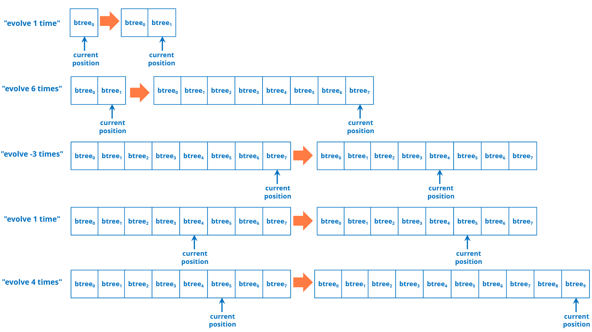
(click on the image above to enlarge it)

Input syntax

Input will be passed to the program through the command line.

  • The first line will be an integer expressing the transition function.
  • The second line will be a serialised cellular automaton binary tree.
  • The third line is an integer expressing the number of queries.
  • The subsequent lines will be as many as the number of queries as per the above.
  • Each query has the following syntax: <integer> <path expression>

The program must interpret the integer in the queries as explained above (Historisation of past states), read the state of the node denoted by the root-based traversal path in the same query, and print it to the standard output before processing the next query.

Example

23749
((X . .) X (X . X)) X ((. X X) . (. X .))
7
3 []
2 [><]
-1 [<>]
-1 [<><]
12 [<<<]
-2 [>><]
1 [>>>]

Assumptions

In this exercise we can safely assume that the traversal paths will be valid and that the history will not be explored before the start of time (generation zero).

We now have the conceptual framework required to start with the implementation. Let’s code!!!

Defining a node in the binary tree

sealed trait Status
object On extends Status
object Off extends Status
case class Node(s: Status) {
  override def toString = s match {
    case On => "X"
    case Off => "."
  }
}
object Node {
  val on = Node(On)
  val off = Node(Off)
}

At the moment of writing, website hackerrank.com supports Scala 2, not 3. This is why I have chosen a sealed trait with two objects instead of a simple enumeration to represent the state (Status in the code). In this way we have only two objects to represent the states. Object Status.On represents state live, whereas object Status.Off represents dead.

Class Node is trivial in that only has an attribute which is the state. Companion object Node returns two objects Node.on and Node.off with the obvious meaning. Please note that using objects like this guarantees that the number of instances in memory is strictly under control. If you do not know what is a companion object, please refer to http://www.scala-lang.org

Method toString() is overridden so that the string representation of the states matches the syntax requirements for this exercise.

Defining a cell

The definition of a node above may give the impression that there is no need to define yet another one for a cell. However, for reasons which will be clearer later, I will define a cell as a class with four attributes: a parent node, its own node, its left child node, and its right child node.

case class Cell(parent: Node, self: Node, left: Node, right: Node)

This definition will make the application of the transition function (the rule) simpler.

Defining a binary tree

Now that we have a node, we can easily define a binary tree.

case class BTree(n: Node, left:Option[BTree], right: Option[BTree])

A binary tree is defined as a structure formed by a node and two optional child trees. But before we delve deeper into the implementation of the BTree, we need to introduce the notion of a Rule.

Defining the rules

case class Rule(r: Char)

A rule is a Char. At this point you may be wondering why. The reason is that, as we have seen above, rules are sequences of 16 values (on/off, or live/dead, etc.). Char in Scala is an unsigned integer of exactly 16 bits. Therefore, it is an extremely compact way to encode a transition function (or a rule, using hackerrank’s terminology).

We can continue with the implementation of rules, by preparing useful data structures by means of the Rule companion object:

 object Rule {
      val nodeTypes = Vector(Node.off, Node.on)
      val sortedCells = nodeTypes.flatMap(n0 => nodeTypes.flatMap(n1 => nodeTypes.flatMap(n2 => nodeTypes.map(n3 => Cell(n0, n2, n1, n3)))))
      val ruleIndex: Map[Cell, Int] = sortedCells.indices.map(i => (sortedCells(i) -> i)).toMap
      val bits: Vector[Char] = (1 to 16).map(n => pow(2, n-1).toChar).toVector
    }

The above needs some explaining.

  • nodeTypes is an ordered sequence of node types modelled as a Vector (please note that no new instance of Node has been created, we are using the singletons defined above).
  • sortedCells is an ordered sequence of all the possible Cells created by generating all the combinations of off and on, and creating a Cell for each of them paying attention to the sort order defined by the author of this exercise who specifies that:
    • The state of the parent node comes first
    • The state of the left child node comes second
    • The state of the node whose new value we are computing comes third
    • The state of the right child node comes fourth
  • ruleIndex is a map which for every possible Cell returns the index of the value in the rule (please refer to the explanation above on how the rules are modelled).
  • bits is a Vector which for every bit index in the rule gives the corresponding binary representation of the on flag. For example, at position 0 it gives 0000000000000001. At position 1 it gives 000000000000010 and so on until position 15 where we have 1000000000000000.

We will better understand the use of the above when we will see how a rule is applied to a binary tree to evolve it to the next generation.

Applying a rule to a cell

case class Rule(r: Char) {
  def applyTo(c: Cell): Node = if ((bits(ruleIndex.getOrElse(c, -1)) & r) > 0) Node.on else Node.off
}

Let us assume that we are now applying a rule to a specific cell. Thanks to the plumbing above the implementation is trivial. First we look for the index in the rule where the new value of the cell is specified. In order to get this index we just have to use our map ruleIndex which contains all the possible cells (key) and their indexes (value). Once we know this index, we get the binary representation of an on flag (a 1) and we compute the logical AND of this flag with the value specified in the rule. If the result of this logical AND is different from 0 than the new state is on, otherwise it is off. This is illustrated by the following picture:

Rule applied to a cell

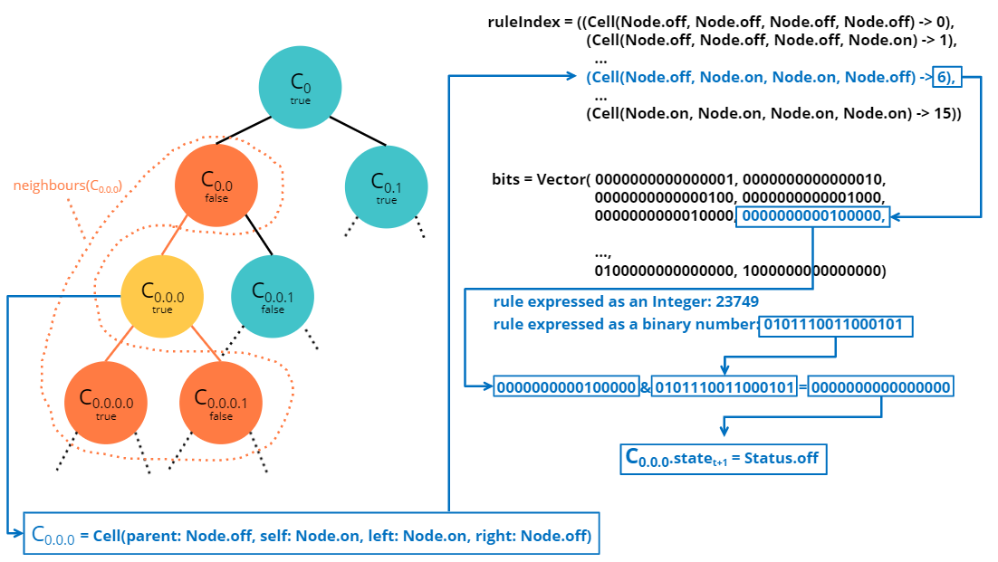
click on picture to enlarge

Remark

You will have noticed that I have used method getOrElse() and may be wondering why, given that by construction, I know that I will find my cell (given that ruleIndex contains all the possible cells). The reason is that the compiler does not know that the operation is safe because a get() on a map in general can fail. Therefore I return -1 in case the cell is not found (which cannot happen).

Applying a rule to the entire tree

case class BTree(n: Node, left:Option[BTree], right: Option[BTree]) {

     def applyRule(r: Rule, parent: Node = Node.off): BTree = {
       def nextCell(o: Option[BTree]) = o match {
         case Some(t) => t.n
         case None => Node.off
       }
       def subTree(o: Option[BTree]) = o match {
         case Some(t) => Some(t.applyRule(r, n))
         case None => None
       }
       BTree(r.applyTo(Cell(parent, n, nextCell(left), nextCell(right))), subTree(left), subTree(right))
     }

Method BTree.applyRule() above generates the next generation tree one node at a time by traversing itself recursively and computing the new state of each and every node.

Please note that the value of parameter parent is set to Node.off by default. This is useful because we start from the root of the tree which, by definition, does not have a parent node. You may wonder why than assign Node.off? The reason is that this is the desired behaviour specified by the author of this programming exercise. Let us now focus on the recursion. First, we need to identify the base case. Then, we must identify the recursion step. We will proceed using structural recursion. The base step is of course the node. We already know how to apply a rule to a node, we have seen it above. What we still need to add is that when a node does not have its parent (root) or one or two child nodes, we will assign default node Node.off. Again, this is the desired behaviour as per specs of this exercise. See The Tree of Life Pro for details (including discussion forums). The step is defined as follows: the new generation of:

BTree(n: Node, left: Option[BTree], right: Option[BTree])

is a new BTree having:

  • its node transformed by rule r: r.applyTo(Cell(parent, n, nextCell(left), nextCell(right)))
  • its sub trees t having node n recursively transformed applying rule r: t.applyRule(r, n)

Remarks

  • we use method def nextCell(o: Option[BTree]) to find the node of sub-trees, so that in case there is none, we can assign default value Node.off
  • we use method def subTree(o: Option[BTree]) to transform a sub-tree, because in case there is none, we just return None instead of starting a new recursive call

If you do not know what is Option[T] in Scala and the meaning of Some(), None, please refer to http://www.scala-lang.org

Now that we know how to transform a binary tree, we are ready to write a method which reads the state of any node given a correct root-based path expression.

Reading the state of a node

  case class BTree(n: Node, left:Option[BTree], right: Option[BTree]) {
     @tailrec
     final def readNode(path: List[Char]): Node = path match {
       case Nil => n
       case h :: pp => val next = h match {
           case '<' => left
           case '>' => right
           case _ => None
         }
         next match {
           case Some(t) => t.readNode(pp)
           case None => n
         }
     }
  }

Remark

We have seen above that the syntax of a path used in the queries is an arbitrary sequence of ‘<‘ and ‘>’ symbols enclosed by ‘[‘ and ‘]’. Method readNode() expects the path to be without any enclosing square brackets, only a sequence of ‘<‘ and ‘>’.

Method readNode() uses the character at the current position in the path to determine if the tree traversal must continue to the left or to the right, and proceeds recursively passing the path without the character just processed to the selected child tree.

Error management

  • if the path is empty than return the current node
  • if there is an unexpected character in the path (neither ‘<‘ nor ‘>’), than return the current node

Annotation @tailrec

You may have noticed that method readNode() has annotation @tailrec. If you do not know what it means, it is a property denoting recursive algorithms satisfying stricter conditions which allow the compiler to generate very efficient code, which makes the runtime performance of this type of recursion comparable to the performance of traditional loop control structures. In other words, you will not have to worry about the recursion running too deep and the method running out of stack. You may find better definitions of a tail recursive algorithm but, for the purposes of this article, I will just say that the intuitive notion entails ending the method with the recursive call. The recursive call is the very last thing which the method does.

Writing the parser

Above we said that the input has a syntax exemplified by this excerpt:

23749
((X . .) X (X . X)) X ((. X X) . (. X .))
7
3 []
2 [><]
-1 [<>]
-1 [<><]
12 [<<<]
-2 [>><]
1 [>>>]

Reading the rule is trivial:

val rule = Rule(readInt.toChar)

Reading the tree and the queries may be a little bit more involved.

Parsing the tree

@tailrec
def getTreeExpr(s: String, expr: String = "", depth: Int=0): (Option[String], String) = {
    if (s.isEmpty) (None, expr + s) else s(0) match {
      case '(' => getTreeExpr(s.substring(1), expr + s(0), depth + 1)
      case ')' => if (depth == 1) (Some((expr + s(0)).trim), s.substring(1))
                     else getTreeExpr(s.substring(1), expr + s(0), depth - 1)
      case c => if (Set(' ', 'X', '.').contains(c))
                  getTreeExpr(s.substring(1), expr + s(0), depth)
                else (None, expr + s)
    }
}

Method getTreeExpr() scans an input string one character at a time checking that only characters defined in the grammar of a tree expression are used (see section above) and that the brackets are balanced.

If a valid tree expression is recognised, it is returned as Some()[String], otherwise None is returned. The remaining part of the input string is also returned along with the recognised tree expression (or None in case of errors).

Please, note that the implementation of this method is also @tailrec.

Building the BTree from a valid tree expression

@tailrec
  def parseNode(s: String): (Option[Node], String) =
    if (s.isEmpty) (None, s) else s(0) match {
      case 'X' => (Some(Node.on), s.substring(1))
      case '.' => (Some(Node.off), s.substring(1))
      case ' ' => parseNode(s.substring(1))
      case _ => (None, s)
    }

  def parseTree(s: String): (Option[BTree], String) =
    if (s.isEmpty) (None, s) else parseNode(s) match {
      case (Some(n), rem) => (Some(BTree(n, None, None)), rem)
      case (None, _) => getTreeExpr(s) match {
        case (None, rem) => (None, rem)
        case (Some(exp), rem) => (BTree(exp), rem)
      }
    }

We will start with method readNode().

  • If symbol ‘X’ is encountered than Some(Node.on) is returned
  • If symbol ‘.’ is encountered than Some(Node.off) is returned
  • If symbol ‘ ‘ (a blank) is encountered than move on to the next char in the string
  • otherwise return None

Whatever the result of the scan, this method returns the remaining part of the input string.

Method parseTree()

  • if the input string is empty, return None
  • if the tree expression denotes a node n, return a BTree with node n and None as left and right sub-trees (leaf node)
  • if the tree expression is not a valid node, parse the input to check if it is a valid a tree expression
    • if not, return None and the input string
    • otherwise build a tree based on the valid tree expression using method def apply(s:String): Option[BTree]

Method def apply(s:String): Option[BTree]

object BTree {
     def apply(s:String): Option[BTree] =
      if (s.length < 7) parseNode(s) match {
          case (Some(n), _) => Some(BTree(n, None, None))
          case _ => None
      } else (s(0), s(s.length - 1)) match {
        case ('(', ')') =>
          val (left, lRem) = parseTree(s.substring(1, s.length - 1))
          val (node, nRem) = parseNode(lRem)
          val (right, rRem) = parseTree(nRem)
          (node, left, right) match {
            case (Some(n), Some(l), Some(r)) => Some(BTree(n, Some(l), Some(r)))
            case _ => None
          }
        case _ => None
      }
  }

Before explaining method apply() it is worth noting that it uses method parseTree() which, as we have seen above, uses method apply(). This situation is called mutual recursion which for a functional programmer is the place “where eagles dare”.

Method apply() uses convenience methods parseNode() and parseTree() to deconstruct a serialised binary tree. From the grammar introduced above we know that a tree is represented as a triplet where the first part is the optional left child tree, the second one is the current node, and the last one is the optional right tree. In order to determine whether the input string must be parsed as a plain node or a binary tree, this method uses a cheap trick: checks the length. This works because we know that the simplest tree is formed by all nodes and has a form similar to “(X . X)” which are seven characters: left bracket, node symbol, blank, node symbol, right bracket. There may be more elegant ways to implement this part, but this works pretty well and is efficient so, for the purposes of this exercise, I will not try to do any better. But, of course, you can!

The apply() method proceeds with structural recursion: if a proper tree expression is recognised, its left and right sub-trees are recursively inspected, until the entire expression is processed, or an error is encountered.

We are now ready for the implementation of the parser for the queries.

Parsing the queries

We have seen above that queries have syntax exemplified by these expressions:

3 []
2 [><]
-1 [<>]
-1 [<><]
12 [<<<]
-2 [>><]
1 [>>>]

Parsing the first part is trivial: it is a signed integer. More interesting is parsing the second part. Here, I will use a regular expression.

def parseQuery(s: String): (Int, String) = {
    import scala.util.{Failure, Success, Try}
    val params = s.split(" ")
    if (params.length != 2) (0, "")
    else {
      val n = Try(params(0).toInt) match {
        case Success(n) => n
        case Failure(_)  => 0
      }
      val regex = "^\\[[<>]*\\]$".r
      val path = if (regex.matches(params(1))) params(1).substring(1, params(1).length-1)
                 else ""
      (n, path)
    }
  }
  • the query is first split using blank as the separator
  • the conversion of the first token to Int is then attempted using functional construct Try instead of imperative exception handling.
  • if the path expression is correct, the enclosing square brackets are removed. This is achieved using params(1).substring(1, params(1).length-1) which omits the first and last character.

Processing the input

def main(args: Array[String]): Unit = {
    val rule = Rule(readInt.toChar)
    BTree(readLine()) match {
      case Some(t) =>
        val nrQueries = readInt()
        assert(nrQueries > 0)
        processInput(nrQueries, rule, Hist(t))
      case None => System.exit(-1)
    }
  }

Method main() is very simple. First, it reads the rule and saves it as a Char. Then, it reads the serialised tree and tries to build a BTree based on it. The test cases run by hackerrank are guaranteed to be syntactically correct. So, we do not have to worry about invalid tree expressions.

After that, the number of queries is read. The core of the algorithm is implemented in method  def processInput(nQueries: Int, rule: Rule, acc: Hist): Unit

@tailrec
  def processInput(nQueries: Int, rule: Rule, acc: Hist): Unit = if (nQueries > 0) {
      val (offset, path) = parseQuery(readLine())
      val h = perform(offset, rule, acc)
      println(h.hist(h.ix).readNode(path.toList).toString())
      processInput(nQueries - 1, rule, h)
  }

This method runs nQueries times and every time reads a query from the command line, processes it, and prints the result to the standard output.

Remark

In imperative languages, instead of writing tail-recursive method processInput() one would have written a simple loop (for or while) using modifiable data structures. The beauty of functional programming is that we can write equivalent code to the imperative which is equally efficient (being @tailrec) without dangerous side effects thanks to the use of immutable data.

Before looking into the perform() method we need to see how the history is implemented and how it works.

The history class

case class Hist(ix: Int, hist: Vector[BTree])
  object Hist {
    def apply(t: BTree): Hist = Hist(0, Vector(t))
  }

We have seen above how the generations of transformed trees are persisted. This data structure contains all the transformations up to the previous generation, along with the position in the history. This is necessary because queries may require us to go back to the past (but not beyond generation 0)

Please note the convenience method apply() which, given a BTree, builds a history object initialised with this tree and an index at position 0.

Method perform()

 def perform(offset: Int, rule: Rule, h: Hist): Hist = {
    assert(h.hist.nonEmpty)
    @tailrec
    def run(times: Int, acc: Vector[BTree] = Vector.empty[BTree]): Vector[BTree] =
      if (times < 1) acc
      else run(times - 1, acc :+ acc.last.applyRule(rule))

    val newIx = h.ix + offset

    if (newIx < 0) h
    else if (newIx < h.hist.length) Hist(newIx, h.hist)
    else Hist(newIx, run(offset - (h.hist.length - h.ix - 1), h.hist))
  }
  • If the offset requires us to move to a position beyond the end of the existing history, method perform will apply the rule to the latest tree as many times as is required to fill the gap in the history.
  • If instead the offset falls within the history, the entire history is returned, along with the new position determined by adding the offset to the previous position.

The updated history returned by method perform() allows method processInput() to print the result to the standard output using this simple statement: println(h.hist(h.ix).readNode(path.toList).toString())

This completes the explanation of the implementation. I hope you have enjoyed this article and have learned something useful. If you have found mistakes you can let me know using the contact form. Please consider that this article and the source code are provided as is. I write this content to the best of my knowledge but there is no guarantee that it is correct or otherwise suitable for any purpose.

Code of conduct

This content aims at making you a better programmer, but you may not use it to gain undeserved credits in programming challenges on any web site. If you want to take programming challenges, please write your own code and do not copy and paste this code because it is against the code of conduct.

Ok, enough with burocracy

If you came this far with this article you deserve a little treat. Here is my code on github:

https://github.com/maumorelli/alaraph

Thank you for reading and up Scala!!!

Matrix Rotation – Functional Implementation in Scala

Introduction

Matrix rotation is the transformation based on replacing the value of a cell with the value of an adjacent one, where the notion of “adjacent” is expressed with reference to the decomposition of a matrix in “rings”. It’s a bit like peeling an onion. Let us consider the matrix depicted above. We can easily identify its outer ring. { a00, a01, a02, a03, a04, a14, a24, a34, a33, a32, a31, a30, a20, a10 }. The next ring is also easily identified: { a11, a12, a13, a23, a22, a21 }.

Assumptions

In this article I will assume that matrix rotation is applied counterclockwise. Similar arguments apply if the rotation is done clockwise. For simplicity’s sake, I will use a matrix of integers.

Representing a matrix

The typical representation of a matrix is based on two-dimensional arrays. Since we will use Scala and we want to learn to write clean algorithms without side effects, we will use immutable type Vector instead.

So, our matrix of integers will be defined as matrix: Vector[Vector[Int]]

The algorithm

I will illustrate the algorithm in steps. First will I explain how the decomposition of a matrix in rings simplifies the logic of rotation. Second, I will explain how to implement this logic without duplicating the content of the matrix for the creation of its constituent rings: we will create an abstraction which will allow us to navigate the matrix as if it were structured in rings. This trick will reduce the space complexity of the algorithm.

Using the rings to implement rotation

Given the matrix in our example above, we can represent the rings using vectors:

val ring0 = Vector( a00, a01, a02, a03, a04, a14, a24, a34, a33, a32, a31, a30, a20, a10 )

val ring1 = Vector( a11, a12, a13, a23, a22, a21 )

As you can see, we have ring0.size = 14 and ring1.size = 6

The logic of rotation can now be expressed using plain modulo arithmetic. If we define “r” the number of (anticlockwise) rotations, and “i” the position of a cell in vector ring0, the new value of ring0(i) is the value of cell ring0((i+r) % ring0.size)

Let us now set r=1

ring0(0) = ring0((0+1) % 14) = ring0(1) = a01

ring0(1) = ring0((1+1) % 14) = ring0(1) = a02

ring0(13) = ring0((13+1) % 14) = ring0(0) = a00

The logic above can be written like this:

(0 until ring0.size).map(i -> ring0((i+r) % ring0.size))

where the “map” method applies the function passed to it as an argument to each element of the collection.

If we apply the logic above to each ring of the matrix, we obtain the rotated matrix.

Implementation

Given a matrix, we have seen above that we can conceptualise it as a set of concentric rings (remember the onion metaphor). We will now write our first method, which will generate a Vector allowing to navigate the matrix as a ring of depth “r”, where depth is 0 for the outer ring.

def m2ring(matrix: Vector[Vector[Int]])(offset:Int): Vector[(Int, Int)] = {
    val m = matrix.size
    val n = matrix(0).size
    val north = (0 + offset to n - 1 - offset).map(j => (offset, j)).toVector
    val east = (1 + offset to m - 2 - offset).map(j => (j, n - 1 - offset)).toVector
    val south = (n - 1 - offset to 0 + offset by -1).map(j => (m - 1 - offset, j)).toVector
    val west = (m - 2 - offset to 1 + offset by -1).map(j => (j, offset)).toVector
    north ++ east ++ south ++ west
  }

If we invoke method m2ring passing our example matrix above, with offset = 0 (this is how the ring depth is called in the method signature), we get this output:

Vector( (0,0), (0,1), (0,2), (0,3), (0,4), (1,4), (2,4), (3,4), (3,3), (3,2), (3,1), (3,0), (2,0), (1,0) )

If we invoke m2ring(matrix)(1) we get:

Vector( (1,1), (1,2), (1,3), (2,3), (2,2), (2,1) )

Our next method will invoke m2ring for each ring depth until the entire matrix is processed (the entire onion is peeled). This method will return two data structures:

  • A Vector of vectors. This vectors will have as many elements as there are rings in the matrix. For each ring, say “i”, rings(i) is the vector having as many elements as there are cells in ring “i”, each element being the (row, col) coordinates of the cell in the matrix.
  • A map having key (row, col) and value (index1, index2) where:
    • (row, col) are the coordinate of a cell in the matrix
    • index1 is the index of the rings vector corresponding to the ring where cell (row, cell) belongs
    • index2 is the index of vector rings(index1) corresponding to the position of cell (row, cell)
def m2rings(matrix: Vector[Vector[Int]]) = {
    val m = matrix.size
    val n = matrix(0).size
    val g = m2ring(matrix)(_)
    val rings = (0 to Math.min(m,n)/2-1).map(i => g(i))
    val coords = (0 until rings.size).flatMap ( i => (0 until rings(i).size).map ( j => rings(i)(j) -> (i, j))).toMap
    (rings, coords)
  }

If we invoke m2rings passing our example matrix above we obtain:

rings = Vector(Vector( (0,0), (0,1), (0,2), (0,3), (0,4), (1,4), (2,4), (3,4), (3,3), (3,2), (3,1), (3,0), (2,0), (1,0) ), Vector( (1,1), (1,2), (1,3), (2,3), (2,2), (2,1) ) )

coords = Map ( (0,0) -> (0,0), (0,1) -> (0,1), (0,2) -> (0,2), (0,3) -> (0,3), (0,4) -> (0,4), (1,0) -> (0,13), (1,1) -> (1,0), (1,2) -> (1,1), (1,3) -> (1,2), (1,4) -> (0,5), (2,0) -> (0,12), (2,1) -> (1,5), (2,2) -> (1,4), (2,3) -> (1,3), (2,4) -> (0,6), (3,0) -> (0,11), (3,1) -> (0,10), (3,2) -> (0,9), (3,3) -> (0,8), (3,4) -> (0,7) )

We have now all the elements to implement the matrix rotation method:

  def perform(matrix: Vector[Vector[Int]], times: Int) = {
    val (rings, coords) = m2rings(matrix)
    def rotateMatrix(lmat: List[Vector[Int]], acc: Vector[Vector[Int]], row: Int = 0): Vector[Vector[Int]] = lmat match {
      case Nil => acc
      case r::rr =>
        val rotatedRow = (0 until r.size ).map { case col =>
                      val (rix, vix) = coords.getOrElse((row, col), (0,0))
                      val (_r, _c) = rings(rix)((vix+times) % rings(rix).size)
                      matrix(_r)(_c)
                    }.toVector

        rotateMatrix(rr, acc :+ rotatedRow, row + 1)
    }
    rotateMatrix(matrix.toList, Vector.empty, 0)
  }

The complete source code for this algorithm is available on my github space.

I hope you enjoyed this article and, up Scala!!!

Solving the Klotski puzzle in Scala

https://upload.wikimedia.org/wikipedia/commons/8/84/Hakoiri3.jpg

Klotski puzzle, Wikimedia

A very good description of the Klotski puzzle is available on programming website Hackerrank. A brief description is given here for convenience’s sake.

What is Klotski

Klotski is a puzzle consisting in a rectangular board containing labelled blocks. These blocks can slide in the four directions up/down/left/right, but they can neither overlap, nor exit the board.

One of these blocks is called the target. Objective is to find the shortest sequence of moves (path) allowing to place the target block in a given location. Any equally short sequence is deemed equivalent.

In counting the moves, subsequent slides of the same block are all counted as one move.

Why is Klotski a challenging programming problem?

Solving the problem requires the ability to reduce unnecessary intermediate configurations which would otherwise lead to a fast explosion of cases to be examined. Although the problem remains intrinsically hard, it is possible to implement optimised algorithms able to solve puzzles requiring n < 200 moves. I tried to find mathematically rigorous proofs of the complexity of known Klotski solver algorithms, but I could not find one. Or at least, none was proved.

The required optimisations to tackle puzzles of the complexity explained above are a very good learning opportunity for programmers who want to learn algorithms, functional programming, recursion, hashing, and many more skills. I have chosen Scala to solve the problem because it allows to write code without side effects, which is particularly suited to teaching good programming practices.

Let’s start from the data structures

I will introduce some basic terms. The picture below represents a Klotski board with five blocks (A, B, C, D, and E). Empty cells are denoted with “.” characters.

Labels need not be single letters, they can be arbitrary strings. If labels have length L > 1, empty cells are denoted by sequences of L “.” characters. For example, the board depicted below is equivalent (isomorphic) to the board above.

We will start from the representation of a Cell.

 case class Cell(y: Int, x: Int) {
    def applyOffset(o: Offset) = Cell(y + o.dy, x + o.dx)
    override def toString = "(%d,%d)".format(y, x)
  }

Cell is a case class and this allows us to write expressions like Cell(2, 3) without having to explicitly invoke a constructor. I have overridden the “toString” method bacause I want an object like Cell(2, 3) to be rendered as “(2, 3)” instead of the default “Cell(2, 3)”. Additionally, I have defined method “applyOffset” which not surprisingly applies an offset to a Cell.

Remark

Please note that Scala is (also) a functional language and the philosophy is to have immutable objects. Therefore, applying an offset to a Cell creates a new Cell, leaving the original one unchanged.

Similarly, we define case class Offset.

  case class Offset(dy: Int, dx: Int) {
    def invert = Offset(-dy, -dx)
  }

This is a trivial class which I will not comment further. A slightly more interesting class is Board.

  case class Block(symbol: String, cells: Set[Cell]) {
    private def minmaxXY = {
      val xx = cells.map { case Cell(_, x) => x }
      val yy = cells.map { case Cell(y, _) => y }
      (xx.min, xx.max, yy.min, yy.max)
    }

    val (minX, maxX, minY, maxY) = minmaxXY
    val uL = Cell(minY, minX)
    val bR = Cell(maxY, maxX)
    val width = maxX - minX + 1
    val height = maxY - minY + 1
  }

A Block is modelled as a set of cells, labelled with a symbol.

Method “minmaxXY” extracts the maximum and minimum X and Y coordinates from the cells. Val xx is built by extracting only the x coordinate from each Cell. The same applies to val yy, mutatis mutandis. An important derived attribute, which we will use to denote the position of a block, is its upper left corner, “uL”.

Remark

It is important to notice that the “uL” cell need not be inside the block itself. For example, let us consider L-shaped block A below. Its upper left cell is Cell(0, 0) which does not belong to the block Block(“A”, Set(Cell(0, 1), Cell(1, 1), Cell(2, 0), Cell(2, 1))

  0 1 2 3 
0 . A . .
1 . A . .
2 A A . .
3 . . . .

We will now model the concept of a move: when a block slides from a certain position to another position, we will log these bits of information:

  • Symbol
  • Upper left cell of the starting position
  • Upper left cell of the ending position

Let us make an example. In the board below we will slide block A:

  0 1 2 3        0 1 2 3
0 . A . .      0 . . . A
1 . A . .  =>  1 . . . A
2 A A . .      2 . . A A
3 . . . .      3 . . . .

The move will be represented with Move(“A”, Cell(0, 0), Cell(0, 2).

case class Move(block: String, from: Cell, to: Cell) {
    def offset = Offset(to.y - from.y, to.x - from.x)
  }

Case class Move has method “offset” which allows to derive the offset applied to Cell “from” to get to Cell “to”.

Building a Board

A board is given in input as a text. The format is illustrated with an example:

5 4
. A B B
. A B B
A A C .
D D C .
D . . E

On the first row we have the number of rows and the number of columns (5 and 4 respectively). Every cell is represented by its symbol and cells are spaced with a blank. We are now ready to define case class Board.

case class Board(blocks: Map[String, Block], block:String, maxX: Int, maxY: Int) {
    val minX = 0
    val minY = 0
    val symbols = blocks.keys
    ...
}

A Board is a map of symbols pointing to their respective block. The special block is saved in property “block”. maxY and maxX have the obvious meaning, but remember that the count starts from 0. In order to create a Board starting from the text input we will create a builder method in the companion object. Remember that in Scala every class can have a companion object with the same name, which is a singleton. See Scala’s documentation on http://www.scala-lang.org for more details.

  object Board {
    def build(b: Vector[Vector[String]], block:String) = {
      val maxY = b.size - 1
      val maxX = b(0).size - 1
      val eb = "." * b(0)(0).length //empty block
      val flatb = for { i <- 0 to maxY
                        j <- 0 to maxX
                        if b(i)(j) != eb
      } yield (b(i)(j), Cell(i,j))

      Board(flatb.groupBy(_._1).map {
        case (y, zz) => (y, Block(y, zz.map(_._2).toSet))
      }, block, maxX, maxY)
    }
  }

“maxY” is set to the number of rows minus 1 (0-referenced). Likewise, “maxX” is set to the number of columns minus 1. Constant “eb” is built by concatenating as many times the “.” character as the length of the symbols in this particular board. The “for” loop goes through the Vector and for every Cell with a symbol different than the empty cell, yields a tuple containing the symbol and the Cell where the symbol was found. The result of this scan is saved in value “flatb”. If we take our example above (copied here for convenience’s sake), this will be the result:

. A B B
. A B B
A A C .
D D C .
D . . E
val flatb = Seq[("A", Cell(0, 1)), ("B", Cell(0, 2)), Cell("B", Cell(0, 3)),
                ("A", Cell(1, 1)), ("B", Cell(1, 2)), Cell("B", Cell(1, 3)),
                ("A", Cell(2, 0)), ("A", Cell(2, 1)), Cell("C", Cell(2, 2)),
                ("D", Cell(3, 0)), ("D", Cell(3, 1)), Cell("C", Cell(3, 2)),
                ("D", Cell(4, 0)), ("E", Cell(4, 3))]

What do we need to do to get from the above to the format required to build a block? Function “groupBy” is the answer. See how it works.

flatb.groupBy(_._1).map {
case (y, zz) => (y, Block(y, zz.map(_._2).toSet))
}

Let’s do it step by step.

flatb.groupBy(_._1)= Map[("A", IndexedSeq[("A", Cell(0, 1)), 
                                          ("A", Cell(1, 1)), 
                                          ("A", Cell(2, 0)), 
                                          ("A", Cell(2, 1))]),
                         ("B", IndexedSeq[("B", Cell(0, 2)), 
                                          ("B", Cell(0, 3)), 
                                          ("B", Cell(1, 2)), 
                                          ("B", Cell(1, 3))]),
                         ("C", IndexedSeq[("C", Cell(2, 2)), 
                                          ("C", Cell(3, 2))]),
                         ("D", IndexedSeq[("D", Cell(3, 0)), 
                                          ("D", Cell(3, 1)), 
                                          ("D", Cell(4, 0))]),
                         ("E", IndexedSeq[("E", Cell(4, 3))])                                  

The subsequent invocations of the “map” method do the following:

  • Create a Block based on each symbol and the sequence of Cells of which the block is composed
  • Convert sequences of Cells into sets of Cells

Performing a move

Performing a move means to slide a block in one of the four admissible directions up/down/left/right. However, some moves are invalid:

  • Moves taking a block out of the board
  • Moves making a block overlap with other blocks

We will now implement the “perform” method which will demonstrate how efficient is the chosen data structure for the definition of the required logic.

 case class Board(blocks: Map[String, Block], block:String, maxX: Int, maxY: Int) {
    val minX = 0
    val minY = 0
    val symbols = blocks.keys

    def perform(s: String, o: Offset) = {
      val b = blocks(s)
      val cells = b.cells.map(c => c.applyOffset(o))
      val outOfBound = cells.find { case Cell(y, x) => y < 0 || y > maxY || x < 0 || x > maxX }

      outOfBound match {
        case Some(_) => None
        case None => val otherBlocks = blocks - s
          val overlap = otherBlocks.values.find(_.cells.intersect(cells) != Set.empty)
          overlap match {
            case Some(_) => None
            case None => Some(Board(blocks + (s -> Block(s, cells)), block, maxX, maxY))
          }
      }
    }
  (...)
 }

Given a Board b, performing a move requires the specification of which block we want to move and in which direction. The block is denoted by its symbol. The direction of the move is denoted by the equivalent offset. The four cardinal directions are denoted by the following offsets:

One move to the left  => Offset( 0, -1)
One move to the right => Offset( 0,  1)
One move upwards      => Offset(-1,  0)
One move downwards    => Offset( 1,  0)

Lets us now consider our example again. Let “brd” be the board depicted below.

. A B B
. A B B
A A C .
D D C .
D . . E

brd.perform(“C”, Offset(0, 1))

will generate this new board:

. A B B
. A B B
A A . C
D D . C
D . . E

Line 8 of code snipped above applies the offset to every cell belonging to the moving block. Line 9 checks whether or not cells exist which after the move go out of the board. In the affirmative case, the result of the move is Option.None (if you do not know what is Option in Scala, please refer to http://www.scala-lang.org).

The second and last check is whether or not the cells of the moved block overlap with the cells of any other block. Please note that the overlap check is elegantly implemented with the Set.intersect method. If the move succeeds, the perform method returns Some(Block).

For the moment we will leave the implementation of class Board. Later in this paper I will come back to it because we will see a magic one-liner which will make the difference between failing and succeeding the demanding performance requirements tested by http://www.hackerrank.com. This single one liner has costed me sleepless nights 🙂

Resist the temptation to look ahead, we have a lot more funny stuff before then.

Laying the ground for the algorithmic approach

I will use this paper to teach you how to write recursive code in Scala, which is an integral part of the functional programming approach. Please note that although recursion has a bad reputation in imperative languages because it consumes precious resources like the stack, the Scala compiler can generate very efficient code, virtually as efficient as a while cycle, on condition that recursion is “tail recursion”, that is, the statement invoking the same method is the very last statement of the method. If you learn to think in terms of recursion, you will be able to write clean code without side effects which uses primarily unmodifiable data. One of the key data structures every Scala programmer must master is List. We will now show how to use lists as a foundational block in our functional approach to solving Klotski. But before then, we need to model the internal states of the Klotski solver. We will now consider the following example.

3 3
A . B
C . B
C D .
A
2 2

The example above has the same syntax we have already described, except for the last two rows, which specify the target: move block “A” to position Cell(2, 2) with the lowest number of moves.

For each configuration our algorithm will do the following:

  • For every symbol, move it around in every possible direction until no more valid moves are possible, avoiding duplicate states (if a move gets to a board which was already generated, the move is discarded)
  • When moving the special block, check if the board is a solution to the problem
  • Add every new board to the history
  • Add all new board generated during this step to the set of boards which have to be explored at the next iteration.

Proposition

The first board generated which is a solution to the puzzle, is the shortest path to the solution.

Since we are exploring the space of solutions stepwise (every step increases the number of moves of one unit), the proposition is trivially true.

Remark

Above we observed that at every step we must add the new boards generated to the set of boards which have to be explored at the next iteration. However, this is not enough. We have a gap in our data model in that, in order to describe the solution, we also need to save the path to each board (the sequence of moves which brings us from the initial board to the desired state in the minimum number of steps. We will call this object a Trail and we will define it as a Board and the Path which has generated it starting from the initial position. Before giving the details, I will show an excerpt of the internal states of our solver. Numbered boards are our “history”. At each iteration, for every symbol all possible moves are tried, avoiding duplicates. This will proceed recursively, as we will see.

1 Move
                                          
A . B       Move(A,(0,0),(0,1))    . A B
C . B  (0) --------------------->  C . B  (1)
C D .                              C D .

A . B       Move(A,(0,0),(1,1))    . . B
C . B  (0) --------------------->  C A B  (2)
C D .                              C D .

A . B       Move(B,(0,2),(0,1))    A B .
C . B  (0) --------------------->  C B .  (3)
C D .                              C D .

A . B       Move(B,(0,2),(1,2))    A . .
C . B  (0) --------------------->  C . B  (4)
C D .                              C D B

A . B       Move(D,(2,1),(1,1))    A . B
C . B  (0) --------------------->  C D B  (5)
C D .                              C . .

A . B       Move(D,(2,1),(0,1))    A D B
C . B  (0) --------------------->  C . B  (6)
C D .                              C . .

A . B       Move(D,(2,1),(2,2))    A . B
C . B  (0) --------------------->  C . B  (7)
C D .                              C . D

2 Moves

. A B       Move(B,(0,2),(1,2))    . A .
C . B  (1) --------------------->  C . B  (8)
C D .                              C D B

. A B       Move(C,(1,0),(0,0))    C A B
C . B  (1) --------------------->  C . B  (9)
C D .                              . D .

. A B       Move(D,(2,1),(1,1))    . A B
C . B  (1) --------------------->  C D B  (10)
C D .                              C . .

. A B       Move(B,(2,1),(2,2))    . A B
C . B  (1) --------------------->  C . B  (11)
C D .                              C . D

(..............................................)

Solution:

A . B   Move(A,(0,0),(1,1))   . . B
C . B --------------------->  C A B
C D .                         C D .

. . B   Move(C,(1,0),(0,0))   C . B
C A B --------------------->  C A B
C D .                         . D .

C . B   Move(D,(2,1),(2,0))   C . B
C A B --------------------->  C A B
. D .                         D . .

C . B   Move(A,(1,1),(2,2))   C . B
C A B --------------------->  C . B
D . .                         D . A

Let us now define the Trail and other useful types.

    case class Trail(board: Board, path: Path)
    type Trails = List[Trail]
    type Offsets = List[Offset]

The Klotski solver algorithm

Based on what we have seen above, the solver is a breadth-first visit of the solution space which explores each individual board generating all the admissible moves symbol by symbol, discarding duplicate states. We can visualize it as a tree whose nodes are Trails (a Board with its Path).

This is the tree of internal states of the solver. Every level down is one more move in the path.

A very handy representation of a breadth-first approach is a list where every subsequent Trail has path with length equal or greater than the one before. In our recursive algorithm it will be built by appending new Trails to the existing list of Boards to be explored.

This is a list representation of the breadth-first visit of the tree. Lists come handy in Functional Programming because they are recursive data structures.

Time has come to read some code.

  def solve(brd:Board, block:String, target:Cell):Path = {
    val symbols = (brd.symbols.toSet - block).toList
    val hist = scala.collection.mutable.Set[Int]()
    val offsets = List(Offset(-1, 0), Offset(1, 0), Offset(0, -1), Offset(0, 1))
    case class Trail(board: Board, path: Path)
    type Trails = List[Trail]
    type Offsets = List[Offset]
 
    (...)

    def _solve(trails: Trails): Path = trails match {
      case t :: tx => val (_trails, _path) =  if (t.path == Nil || 
        t.path.head.block != block) pursueTarget(List(t))
      else (Nil, Nil)
        if (_path != Nil) _path
        else {
          val _symbols =  if (t.path == Nil) symbols
          else (symbols.toSet - t.path.head.block).toList
          val newTrails = checkOneTrail(t, _symbols)
          _solve(tx ++ newTrails ++ _trails)
        }
      case Nil => Nil
    }


    if (isSolved(block, target, brd)) Nil
    else {
      hist.add(brd.hashCode)
      val trails = List(Trail(brd, Nil))
      if (!symbols.isEmpty) _solve(trails) else pursueTarget(trails)._2
    }
  }

The algorithm is driven by the “solve” method, which is invoked passing the Board, the special block symbol, and the target Cell. The “solve” method checks if by chance the initial Board is already a solution (border case). Otherwise it adds the “hashCode” of the Board to the “hist” Set.

The history of explored Boards

I initially implemented the “hist” Set using a more “functional” immutable Set passed as a parameter to “_solve” and all other methods. In this case, however, given the fast increasing size I then consciously decided to compromise on the purity of the implementation to optimise the performance. Since the “hist” Set is only visible inside method “solve”, the risk of undesired side-effects is well controlled. This is an example of how first principles can be consciously traded off if one knows what he/her is doing.

But this is not all. A second design decision is to historise hash codes of the Boards, instead of the Boards themselves. The rationale is again performance (www.hackerrank.com requirements in this regard are strict). It is a lot more efficient to compare integers than to compare entire boards and their blocks, symbols and cells. Of course, the probability of a clash is small when using good hashing algorithms, but its not null (for the very nature of hashes, which generate values in a constrained range from unconstrained inputs). This is the trade-off. It works in practice, but it is not a 100% mathematically sound approach. So, what would happen in case of a clash? A board would be “found” in the history, which was never before really generated and in the worst scenario this could lead to a sub-optimal solution. This never occurred in any of the 26+ http://www.hackerrank.com test cases or even in my own ones.

The hash function

This function is a very critical part of the algorithm: getting it wrong screws up everything else (I am saying it for a reason). So, what’s special about the hash function of a Board and why does not the default “hashCode” function work well enough? The default hashCode implementation in Scala is actually pretty good. But when we run the algorithm using the default implementation we have an exponential explosion of states. I will now illustrate why and how to fix it. Let us consider the following Klotski puzzle.

5 4
A B C .
A D E .
F F G G
F . G .
H I L L
A
3 3

The following Boards all have distinct hashCodes, because they are different. But, are they any different in terms of solving the puzzle? No, they are not, because they have the same exact morphology the only distinction being that same-shaped blocks have different labels, which is not a differentiator for the search of the optimal path.

A B C .   A C B .   A B C .   A B C .   A B C .
A D E .   A D E .   A E D .   A D E .   A D E .
F F G G   F F G G   F F G G   G G F F   F F G G
F . G .   F . G .   F . G .   G . F .   F . G .
H I L L   H I L L   H I L L   H I L L   I H L L

I could list many more equivalent permutations of this Board, but by now you should get the point. So, our hash function will need to generate the same code for all the equivalent Boards, so that they are not unnecessarily explored slowing down the search to unacceptable levels. Or, if you prefer, so that the space of possible solutions is limited to truly relevant configurations. This is how the correct “hashCode” method looks like.

override def hashCode = (blocks(block).hashCode :: (blocks - block).values.map (b => b.cells.hashCode).toList.sorted).hashCode

The equivalent blocks are made to generate the same hash by removing their symbol from the computation. The symbol of the special block is instead maintained because where the special block is located is a differentiating factor. This hashCode function induces an equivalence relation on the set of generated Boards. Reducing the search to the set of equivalence classes makes the complexity of the search manageable with problems of the size defined above (but remains inefficient for problems of arbitrary size).

Coming back to the algorithm, at the core of the “solve” method there is this logic:

  • A trail is explored to see if it is possible to move the special block to the target cell. In the affirmative case the algorithm stops and returns the path.
  • Otherwise, the new configurations are added to the history and are appended to the set of Boards which have to be further explored.
  • The trail is processed by scanning all possible moves of all symbols in order to prepare the boards to be explored at the next iteration. These new configurations are appended to the list of trails to be explored. This sequence is guaranteed to produce a list equivalent to a breadth-first tree traversal (see above).
  • Some further optimisations are applied. For example, if the last move in the path of a given trail involved symbol s, the algorithm will not try to move block s because all possible moves were already tried in the step before.

The below is the implementation of all the other recursive parts of the algorithm, which should be self-explanatory after all the clarifications above.

  def solve(brd:Board, block:String, target:Cell, maxmoves: Int = 250):Path = {
    val symbols = (brd.symbols.toSet - block).toList

    val offsets = List(Offset(-1, 0), Offset(1, 0), Offset(0, -1), Offset(0, 1))
    case class Trail(board: Board, path: Path)
    type Trails = List[Trail]
    type Offsets = List[Offset]


    def moveBlockAroundOnce(trail: Trail, s: String, offsets: Offsets, hist: Set[Board]=Set.empty, acc: Trails = Nil): Trails = offsets match {
      case o :: ox => trail.board.perform(s, o) match {
        case Some(newBoard) => if (hist.contains(newBoard))
          moveBlockAroundOnce(trail, s, ox, hist, acc)
        else
          moveBlockAroundOnce(trail, s, ox, hist+newBoard, Trail(newBoard,
            Move(s, trail.board.blocks(s).uL, newBoard.blocks(s).uL) :: trail.path)::acc)

        case None => moveBlockAroundOnce(trail, s, ox, hist, acc)
      }
      case Nil => acc
    }

    def moveBlockAround(trails: Trails, s: String, hist: Set[Board]=Set.empty, acc: Trails = Nil): Trails = trails match {
      case t :: tx => val _trails = moveBlockAroundOnce(t, s, offsets, hist + t.board)
        moveBlockAround(tx ++ _trails, s, hist.union(_trails.map(t=>t.board).toSet), acc ++ _trails)
      case Nil => acc
    }

    def sanitize(trails:Trails, acc: Trails = Nil): Trails = trails match {
      case t::tx => val hashcd = t.board.hashCode
        if (hist.contains(hashcd)) sanitize(tx, acc)
        else {
          hist.add(hashcd)
          sanitize(tx, t::acc)
        }
      case Nil => acc
    }

    def checkOneTrail(trail: Trail, symbols: List[String], acc: Trails = Nil): Trails = symbols match {
      case s :: sx => val _trails = moveBlockAround(List(trail), s)
        val newTrails = sanitize(_trails)
        checkOneTrail(trail, sx, acc ++ newTrails)
      case Nil => acc
    }

    def pursueTarget(trails: Trails, acc: List[Trail] = Nil): (Trails, Path) = trails match {
      case t :: tx => if (isSolved(block, target, t.board)) (trails, t.path)
      else {
        val _trails = moveBlockAroundOnce(t, block, offsets)
        val newTrails = sanitize(_trails)
        pursueTarget(tx ++ newTrails, acc ++ newTrails)
      }
      case Nil => (acc, Nil)
    }

    def _solve(trails: Trails): Path = trails match {
      case t :: tx => val (_trails, _path) =  if (t.path == Nil || t.path.head.block != block) pursueTarget(List(t))
      else (Nil, Nil)
        if (_path != Nil) _path
        else {
          val _symbols =  if (t.path == Nil) symbols
          else (symbols.toSet - t.path.head.block).toList
          val newTrails = checkOneTrail(t, _symbols)
          _solve(tx ++ newTrails ++ _trails)
        }
      case Nil => Nil
    }


    if (isSolved(block, target, brd)) Nil
    else {
      hist.add(brd.hashCode)
      val trails = List(Trail(brd, Nil))
      if (!symbols.isEmpty) _solve(trails) else pursueTarget(trails)._2
    }
  }

The “history” used in the inner methods is not optimised with hashCodes. I wanted to demonstrate an alternative approach which does not affect the overall performance because it is applied in the context of a very limited and defined part of the algorithm. Still, it is easy to get it wrong (actually, I did, initially) if the filter is applied too early inside the inner recursive methods. The reason is that while we certainly want to discard equivalent boards, we still need to let the algorithm use them to find the set of all possible moves for a given symbol because otherwise we may prematurely cut a path leading to valid boards.

There are of course some more details which you can find in my complete implementation of the Klotski solver in github. Some further optimisations and beautifications are possible, but this implementation passed all the demanding tests in http://www.hackerrank.com. By the way, this paper and the accompanying code is provided as is, with the intent to teach programming techniques. It is explicitly forbidden to misuse it, for example, by cheating in programming challenges or gain undeserved credits.

That said, I hope you enjoyed this paper and I wish you a lot of fun with Scala programming. Up Scala!